Final Exercise: Building a Speech Recognizer and integrating it with the chatbot…!

Update: You can access all the code for the workshop at:

Final Exercise

Use the chatbot, template_matching and speech_processing notebooks to create a voice activated chatbot that answers yes/know questions.

Solution:

  • Use the Bot class and the yes_no_processor to get a ready made chatbot
  • Create a new speech_source for your Bot instance
  • Use the AudioManager from speech_processing to record audio
  • Extract MFCCs for the audio clips corresponding to yes and no
  • Use the Trellis idea from template_matching to recognize yes/no

 Answer

The imports given below are from the previous exercises. You can view all the posts on this topic here.

from collections import defaultdict

import importer
from chatbot import StatementProcessor, get_yes_no_processor, get_keyboard_source, Bot
from template_matching import Trellis
from speech_processing import AudioManager

from python_speech_features import mfcc
from python_speech_features.base import delta
import numpy as np
from collections import defaultdict
import pickle
import os
importing notebook from chatbot.ipynb
importing notebook from template_matching.ipynb
importing notebook from speech_processing.ipynb
if __name__ == "__main__":
    # Install python_speech_features that contains a routine to extract mfcc
    !pip install -U python_speech_features
class TemplateManager:

    @staticmethod
    def build_templates(words=["test", "hello", "welcome", "goodbye"],
                        no_templates=1,
                        output_file="templates.out"):

        audioManager = AudioManager()

        templates = defaultdict(list)

        for word in words:
            for ii in range(no_templates):
                ok = 'n'
                while (ok.lower()=='n'):
                    print("%d/%d Say %s" %(ii, no_templates, word))
                    samples = audioManager.record(2, filter_silence=False)
                    audioManager.play(samples)
                    features = feature_extractor(samples)
                    templates[word].append(features)
                    #ok = raw_input("OK?") # python2
                    ok = input("OK?") # python3
        pickle.dump(templates, open(output_file,"wb"))
    
    @staticmethod
    def get_templates(filename):
        if os.path.exists(filename):
            return pickle.load(open(output_file,"rb"))
        else:
            print("Template file not found.")
def feature_extractor(samples):
    samples = np.concatenate(samples)
    samples = samples/np.abs(samples).max()
    samples = samples - samples.mean()
    mfcc_features = mfcc(samples, samplerate=8000, winlen=0.032, winstep=0.016, numcep=13, appendEnergy=True, preemph=0)
    #features = np.vstack((mfcc_features, delta(mfcc_features, 1)))
    features = mfcc_features
    return features
def scoring_func(x, y):
    #print(x.shape, y.shape)
    #print(x, y)
    return np.abs(x - y).sum()


def get_speech_source(filename):
    # Load speech templates
    # Return a function that can detect speech
    audioManager = AudioManager()
    trellis = Trellis(match_weight=1.0, delete_weight=1.0, add_weight=1.0, scoring_func=scoring_func)
    
    templates_dict = TemplateManager.get_templates(filename)
    statement_processor = StatementProcessor()
    
    def speech_source():
        best_scoring_word = ""
        #inp = raw_input("Start recording?") # python2
        inp = input("Start recording?") # python3
        if len(inp)>0 and inp[0] == "/":
            return inp
        samples = audioManager.record(2, wait_for_kb=False)
        features = feature_extractor(samples)
        
        min_score = 1e9
        min_word = ""
        for word, word_templates in templates_dict.items():
            avg_score = 0.0
            for word_template in word_templates:
                score, bp = trellis.match(word_template, features)
                avg_score += score
            avg_score = avg_score / float(len(word_templates))
            #print(word, avg_score)
            if avg_score < min_score:
                min_score = avg_score
                min_word = word
        print("YOU>> ", min_word)
        return min_word
        # Record some audio
        # Match the audio with every template using Trellis
        # Return the best scoring result 
        return best_scoring_word
    return speech_source
words = ["yes", "no"]
no_templates = 1
output_file = "templates.out"
TemplateManager.build_templates(words, no_templates, output_file)
0/1 Say yes
Press Enter to start recording...
* recording
* done recording
OK?
0/1 Say no
Press Enter to start recording...
* recording
* done recording
OK?
chatbot = Bot(statement_processor=StatementProcessor(statement_logic=get_yes_no_processor()),
             input_source=get_speech_source(output_file))
chatbot.start_bot()
Start recording?
* recording
* done recording
before 125
after 125
YOU>>  yes
[ 0 ] Poincare >>  Is it raining?
[ 0 ] Poincare >>  Give the right answer.
Start recording?
Posted in Programming, SpeechActivatedChatBotWorkshop | Tagged , , , | Leave a comment

Speech processing with Python: Basics…

Update: You can access all the code for the workshop at:

Introduction to Speech Processing

What is a signal?

What can we use speech signals for?

import pyaudio
import threading

class AudioManager:
    def __init__(self,chunk=128, fmt=pyaudio.paInt16, channels=1, rate=8000):
        self.chunk = chunk
        self.fmt = fmt
        self.channels = channels
        self.rate = rate
        self.energy_th = 0

    def build_silence_model(self, duration=1, factor=1.5):
        print("Please stay quiet. Measuring ambient noise...")
        frames = self.record(duration, filter_silence=False, wait_for_kb=False)
        es = []
        for f in frames:
            energy = self.energy(f)
            es.append(energy)
        es = np.array(es)
        self.energy_th = es.mean() + factor*es.std()

    def energy(self, frame):
        return sum([abs(v) for v in frame])/len(frame)
    
    def record(self, duration=1, filter_silence=True, wait_for_kb=True):
        if wait_for_kb:
            #x = input("Press Enter to start recording...") # Python3
            x = raw_input("Press Enter to start recording...")
        p = pyaudio.PyAudio()
        stream = p.open(format=self.fmt,
                        channels=self.channels,
                        rate=self.rate,
                        input=True,
                        frames_per_buffer=self.chunk)
        print("* recording")
        frames = []
        starting_silence = True
        silence_frame_cnt = 0
        for i in range(0, int((self.rate / self.chunk) * duration)):
            data = stream.read(self.chunk)
            d = np.fromstring(data, dtype=np.int16)
            if filter_silence:
                energy = self.energy(d)

                if energy < self.energy_th:
                    if starting_silence:
                        continue
                    else:
                        silence_frame_cnt += 1
                        if silence_frame_cnt == int(self.rate/self.chunk):
                            break
                else:
                    starting_silence = False
                    silence_frame_cnt = 0
            frames.append(d)
        print("* done recording")
        
        stream.stop_stream()
        stream.close()
        p.terminate()
        
        if filter_silence:
            print("before", len(frames))
            term = len(frames)
            for ii in range(len(frames)-1, -1, -1):
                e = self.energy(frames[ii])
                if e < self.energy_th:
                    term = ii
                else:
                    break
            frames = frames[:term]
            print("after", len(frames))
        return frames

    def play(self, frames):
        
        p = pyaudio.PyAudio()  
        #open stream
        stream = p.open(format = self.fmt,
                        channels = self.channels,
                        rate = self.rate,
                        output = True)
        
        if type(frames) is list:
            frames = list(frames)
            b = np.zeros(frames[0].shape, dtype=np.int16)
            frames.insert(0, b)
            frames.append(b)
            frames = np.concatenate(frames)
        
        stream.write(frames.tostring())
        
        #stop stream  
        stream.stop_stream()  
        stream.close()  
        #close PyAudio  
        p.terminate()  

def plot_fft(y, fs):

    n = len(y) # length of the signal
    k = np.arange(n)
    T = 2*n/float(fs)
    frq = k/T # two sides frequency range
    frq = frq[range(int(n/2))] # one side frequency range

    Y = fftpack.dct(y)
    Y = Y[:int(n/2)]
    plt.plot(frq, abs(Y))
    plt.show()


from scipy import signal, fftpack
import matplotlib.pyplot as plt
import numpy as np
import math

if __name__=="__main__":
    # Concept of normalized time and frequency...
    fs = 8000
    Ts = 1/float(fs)
    
    t = np.arange(0, 1, Ts)
    y = np.sin(2*np.pi*200*t) + 0.25*np.sin(2*np.pi*500*t)#+ np.tan(t + 0.5) + 2*np.cos(t + 0.5)
    plt.plot(t, y)
    plt.show()
    plot_fft(y, fs)
if __name__=="__main__":
    audioManager = AudioManager()
    audioManager.build_silence_model(factor=1.1)
    samples = audioManager.record(1, filter_silence=False)
    audioManager.play(samples)
    plt.plot(np.concatenate(samples))
    plt.show()
Please stay quiet. Measuring ambient noise...
* recording
* done recording
Press Enter to start recording...
* recording
* done recording
 
 speech_processing_3
if __name__=="__main__":
    # Speech spectrogram
    f, t, Sxx = signal.spectrogram(np.concatenate(samples),
                                   fs=audioManager.rate,
                                   window=signal.gaussian(audioManager.chunk/2, audioManager.chunk/8),
                                   nperseg=audioManager.chunk/2)
    plt.pcolormesh(t, f, Sxx)
    plt.show()

    f, t, Sxx = signal.spectrogram(np.concatenate(samples),
                                   fs=audioManager.rate,
                                   window=signal.gaussian(audioManager.chunk*2, audioManager.chunk),
                                   nperseg=audioManager.chunk*2)
    plt.pcolormesh(t, f, Sxx)
    plt.show()
if __name__=="__main__":
    print(len(samples))
    print("Voiced Region (Vowel)")
    plt.plot(samples[45])
    plt.show()
    plot_fft(samples[45], fs=8000)
    print("Noise")
    plt.plot(samples[5])
    plt.show()
    plot_fft(samples[5], fs=8000)
62
Voiced Region (Vowel)
Comment -- bad example. will fix later :)
Noise
Posted in Programming, SpeechActivatedChatBotWorkshop | Tagged , , | Leave a comment

Exercise 4: Extending the bot to do QA

Update: You can access all the code for the workshop at:

Exercise 4

  • Re-formulate the chatbot to ask a list of Yes/No questions that is procured from a file.
  • State if the user’s answer is correct or wrong.
  • Make the source of input to the bot configurable. For now, it will come from the keyboard. Soon, we’ll use our voice.

 Answer

This code makes use of the “Context” class created Exercise 3. Click here to view Exercise 3

from collections import deque
from random import choice

class StatementProcessor:
    
    def __init__(self, N=10, statement_logic=lambda context, x: (True, ["OK"])):
            self.context = Context(N)
            self.statement_logic = statement_logic
    
    def process_statement(self, x):
        context = self.context
        if x[0] == "/":
            cont, response = self.process_command(x[1:])
        else:
            cont, response = self.statement_logic(context, x)
        return cont, response

    def process_command(self, x):
        context = self.context
        parts = x.split()
        cmd = parts[0]
        args = parts[1:]
        
        cont = False
        response = []
        
        if cmd == "quit":
            cont = False
            response = ["Goodbye!"]
        elif cmd == "clearcontext":
            context.clear()
            cont = True
            response = ["Cleared context."]
        elif cmd == "printcontext":
            response = context.get()
            response.append("Context length: %d" % (len(context)))
            cont = True
        elif cmd == "resizecontext":
            if len(args) == 1:
                try:
                    context.resize(int(args[0]))
                    cont = True
                    response = ["Resized context to %s" % (args[0])]
                except TypeError:
                    cont = True
                    response = ["Context size should be int"]
            else:
                cont = True
                response = ["resizecontext requires new size (int)"]
        else:
            cont = True
            response = ["Invalid Command"]
        context.add(x, response ,cont)
        return cont, response

    
def get_yes_no_processor(filename="binary_questions.txt"):
        qas = [v.split("#<>#") for v in filter(None, open(filename).read().split("\n"))]
        def statement_logic(context, x):
            prev_context = context.get()
            response = ["OK."]
            cont = True
            if len(prev_context)>0:
                prev_context = prev_context[-1]
            else:
                prev_context = {}
            #print(prev_context)
            if "tags" in prev_context and "question" in prev_context["tags"] and "qtype" in prev_context["tags"]["question"] and prev_context["tags"]["question"]["qtype"] == "binary":
                if prev_context["tags"]["question"]["expected_response"] == x:
                    response = ["Correct."]
                else:
                    response = ["Wrong.","Right answer is %s" %(prev_context["tags"]["question"]["expected_response"])]
                context.add(x, cont, response)
            else:
                qa_current = choice(qas)
                response = [qa_current[0]]
                response.append("Give the right answer.")
                context.add(x, cont, response, question={"expected_response": qa_current[1], "qtype": "binary"})
            return cont, response
        return statement_logic


def get_keyboard_source():
    def read_keyboard():
        #return raw_input("You>> ") # Python2
        return input("You>> ")
    return read_keyboard
    
class Bot:
    def __init__(self, name='Poincare', statement_processor=StatementProcessor(), input_source=get_keyboard_source()):
        self.name = name
        self.statement_processor = statement_processor
        self.input_source = input_source

    def start_bot(self):
        cont = True
        chat_cnt = 0

        while cont:
            x = self.input_source()
            cont, response = self.statement_processor.process_statement(x)
            for r in response:
                print("[", chat_cnt, "]", self.name, ">> ", r)
            chat_cnt += 1
 Running the chatbot
if __name__=="__main__":
    bot = Bot(statement_processor=StatementProcessor(statement_logic=get_yes_no_processor()))
    bot.start_bot()
 Output
You>> Hi
[ 0 ] Poincare >>  Is it cold outside?
[ 0 ] Poincare >>  Give the right answer.
You>> no
[ 1 ] Poincare >>  Correct.
You>> /quit
[ 2 ] Poincare >>  Goodbye!
Posted in Programming, SpeechActivatedChatBotWorkshop | Tagged , | Leave a comment

Exercise 3: Basic chatbot…

Update: You can access all the code for the workshop at:

Exercise 3

Chatbot dialog management

Your job is to create a chatbot… As a first step, you will have to define the chatbot’s framework.

In this exercise, you will have to write the necessary code to:

  1. Read input from a user, as a chatbot would and display a simple response for an input. This should look like a conversation happening on a messenger.
  2. Maintain dialogue state: which is the past “N” inputs from the user to the bot and the bot’s responses
  3. A few housekeeping commands for the bot:
    • Clear the context (/clearcontext)
    • Print out the context (/printcontext)
    • Configure the size of the context (/resizecontext N)
    • Quit the conversation (/quit)

 Answer

from collections import deque

def process_statement_basic(x):
    if x[0] == "/":
        cont, response = process_command(x[1:])
    else:
        response = ["OK."]
        cont = True
    return cont, response


def process_command(x):
    parts = x.split()
    cmd = parts[0]
    args = parts[1:]
    
    
    global context
    if cmd == "quit":
        return False, ["Goodbye!"]
    elif cmd == "clearcontext":
        context.clear()
        return True, ["Cleared context."]
    elif cmd == "printcontext":
        response = context.get()
        response.append("Context length: %d" % (len(context)))
        return True, response
    elif cmd == "resizecontext":
        if len(args) == 1:
            
            try:
                context.resize(int(args[0]))
                return True, ["Resized context to %s" % (args[0])]
            except TypeError:
                return True, ["Context size should be int"]
        else:
            return True, ["resizecontext requires new size (int)"]
    else:
        return True, ["Invalid Command"]

class Context:
    
    def __init__(self, N):
        self.N = N
        self.context = None
        self.init()
    
    def __len__(self):
        return self.N
    
    def init(self):
        if self.context is None:
            self.context = deque(list(), self.N)
        else:
            self.context = deque(list(self.context), self.N)
        
    def add(self, x, response, cont, **kwargs):
        self.context.append({"x": x, "response": response, "cont": cont, 'tags': kwargs})
        
    def clear(self):
        self.context = None
        self.init()
    
    def resize(self, N):
        self.N = N
        self.init()

    def get(self):
        return list(self.context)
        
context = None

def start_chatbot(N = 10, name = 'Poincare'):
    global context
    context = Context(N)
    
    cont = True
    chat_cnt = 0
    
    while cont:
        x = input("You>> ")
        cont, response = process_statement_basic(x)
        for r in response:
            print("[", chat_cnt, "]", name, ">> ", r)
        context.add(x, response ,cont)
        chat_cnt += 1
Running the chatbot…
if __name__=="__main__":
    # Start the bot...  
    start_chatbot()
 Output:
You>> hi
[ 0 ] Poincare >>  OK.
You>> hello
[ 1 ] Poincare >>  OK.
You>> /resizecontext 2
[ 2 ] Poincare >>  Resized context to 2
You>> /printcontext
[ 3 ] Poincare >>  {'x': 'hello', 'tags': {}, 'cont': True, 'response': ['OK.']}
[ 3 ] Poincare >>  {'x': '/resizecontext 2', 'tags': {}, 'cont': True, 'response': ['Resized context to 2']}
[ 3 ] Poincare >>  Context length: 2
You>> /quit
[ 4 ] Poincare >>  Goodbye!
Posted in Programming, SpeechActivatedChatBotWorkshop | Tagged , | 1 Comment

Exercise 2: Spelling correction with Minimum-Edit Distance

Update: You can access all the code for the workshop at:

We’ll be using the “Trellis” class created in Exercise one to implement a simple program to correct spellings. Check here for the “Trellis” class.

Exercise-2

Use the matching algorithm written above to correct spellings of words intput thru the keyboard. I.e. create your own spell checker! (albiet it being quite inefficient…)

A list of english words has been given to you in words2.txt

if __name__=="__main__":
    dictionary = list(filter(None, open("words2.txt","r").read().split("\n")))

    trellis = Trellis(lambda x, y: 0.0 if x == y else 1.0, delete_weight=4.0)
    print("Enter /quit to quit")
    while True:
        x = input("word>> ")
        x = x.lower()
        if x == "/quit":
            print("Goodbye!")
            break
        if x in dictionary:
            print("word found")
            continue
        min_sc = 1e9
        match = x
        for el in dictionary:
            sc = trellis.match(el, x, normalize_score=False)[0]
            if sc < min_sc:
                min_sc = sc
                match = el
        print("closest match: ", match)
Enter /quit to quit
word>> hsllo
closest match:  hello
word>> vase
closest match:  case
word>> /quit
Goodbye!
Posted in Programming, SpeechActivatedChatBotWorkshop | Tagged , | Leave a comment

Exercise 1: Minimum-Edit-Distance (using Dynamic Programming)

Update: You can access all the code for the workshop at:

Exercise-1

Create a class Trellis that

  • takes in four arguments: match_weight, delete_weight, add_weight, and scoring_func.
    • scoring_func is a function that computes the distance or score between two values.
    • match_weight, delete_weight, add_weight are floats that weigh a diagonal, horizontal, and vertical transitions, respectively.
  • contains a method match(X, Y) where X and Y are arrays of values; the values can be characters, scalars, or even vectors that returns the minimum-edit-distance/matching-score between X and Y and the shortest path (as an array of 2-tuples).

Answer

The “Trellis” Class:

import numpy as np
from copy import deepcopy

class Trellis:
    
    def __init__(self, scoring_func, match_weight=1.0, delete_weight=1.0, add_weight=1.0):
        self.scoring_func = scoring_func
        self.match_weight = match_weight
        self.delete_weight = delete_weight
        self.add_weight = add_weight
    
    def match(self, X, Y, normalize_score=True):
        scoring_func = self.scoring_func
        match_weight, delete_weight, add_weight = self.match_weight, self.delete_weight, self.add_weight
    
        score_rows = np.zeros((2, len(X)+1))
        path_counts = np.zeros((2, len(X)+1))
        back_pointers = []
        for ii in range(len(X)):
            back_pointers.append([])
        score_rows[0, 1:] = 1e9
        score_rows[1:, 0] = 1e9
        
        
        jj = 1
        while jj < len(Y) + 1:
            back_pointer_before_iteration = deepcopy(back_pointers)
            for ii in range(1, len(X)+1):
                diag_score = score_rows[0, ii-1] + match_weight
                vert_score = score_rows[0, ii] + add_weight
                horiz_score = score_rows[1, ii-1] + add_weight
                min_score = min(diag_score, vert_score, horiz_score)
                if min_score == diag_score:
                    back_pointers[ii-1] = list(back_pointer_before_iteration[ii-2])
                    back_pointers[ii-1].append( (jj-2, ii -2) )
                    #print("DIAG", ii-1, back_pointers)
                elif min_score == vert_score:
                    back_pointers[ii-1].append( (jj-2, ii-1) )
                    #print("VERT", ii-1, back_pointers)
                else:
                    back_pointers[ii-1] = list(back_pointers[ii-2])
                    back_pointers[ii-1].append( (jj-1, ii-2) )
                    #print("HORIZ", ii-1, jj-1, back_pointers)
                node_total = min_score + scoring_func(X[ii-1], Y[jj-1])
                score_rows[1, ii] = node_total
            score_rows[0, :] = score_rows[1, :]
            score_rows[1, 1:] = 0
            jj += 1
            #print(back_pointers)
        return score_rows[0, -1], back_pointers[-1]
Testing the “Trellis” class
if __name__=="__main__":
    trellis = Trellis(match_weight=0.0, scoring_func=lambda x, y: 0.0 if x == y else 1.0)

    test_cases = [
        ['TEST', 'TES'],
        ['geek', 'gesek'],
        ['ISLANDER', 'SLANDER'],
        ['MART', 'KARMA'],
        ['TEST', "TEST"]
    ]

    for case in test_cases:
        print(case, trellis.match(case[0], case[1], normalize_score=True)[1])
 Output:
['TEST', 'TES'] [(-1, -1), (0, 0), (1, 1), (2, 2)]
['geek', 'gesek'] [(-1, -1), (0, 0), (1, 1), (2, 1), (3, 2)]
['ISLANDER', 'SLANDER'] [(-1, -1), (0, 0), (0, 1), (1, 2), (2, 3), (3, 4), (4, 5), (5, 6)]
['MART', 'KARMA'] [(-1, -1), (0, 0), (1, 1), (2, 2), (3, 2)]
['TEST', 'TEST'] [(-1, -1), (0, 0), (1, 1), (2, 2)]
Posted in Programming, SpeechActivatedChatBotWorkshop | Tagged , | 1 Comment

Python tutorial

Update: You can access all the code for the workshop at:

Introduction to Python


Difficulty level: undergraduate

Objectives:

  1. Learn about Python
  2. Get to speed with writing programs in Python

Introducing Python

Python is:

  • A high-level programming langauge
  • Dynamically, Strongly typed
  • For general-purpose computing
  • Interpreted
  • Automatic/Internal Memory Management
  • Object-oriented, Structural, a “little” Functional and Aspect-Oriented

CPython is an open-source implementation of Python

Was first written in late 1980s by Guido van Rossum.


Advantages of learning Python (over other high-level languages)

  • Generally uses fewer lines of code to express concepts
  • Has libraries for literally anything you can think of (Web, Mobile, Scientific, Data Storage, etc.)
  • Dynamically and strongly typed? Has support for type-hinting
  • More productive; can be used for small to large products; prototyping to production-grade systems
  • Has an open-source implementation

Most linux distributions ship with Python 2.7.

In this course, we’re going to use Python 3.4+. The Python 2 series are scheduled to be deprecated by 2020.


Contents

Basics

  • The “hello world”
  • Basics
    • Variable Assignments
    • Function calls
    • Variable scope
    • Input and Output
    • Exception handling
    • Loops and conditional statements
  • Data Types
    • Mutable and non-mutable types
    • Iterators and Generators
    • Closures
    • Decorators
  • Packaged utilities
    • Collections
    • Itertools
  • A bit of OOP
  • Using external libraries
  • Basic packaging

Application Development Examples

  • A web server
  • Data crunching with numpy and pandas

The “Hello World”


In [2]:
if __name__ == "__main__":
    
    print("Hello World!")
Hello World!

Basics


Variable Assignments

Python uses duck-typing…
It is dynamically, but strongly typed.

x = 2 # int
y = ‘5’ # or y = “5”; String
z = 2.0 # float
t = [1, 2] # This is a list – which is similar to your linked list (more on this later)

print(x + z) # Involves automatic type conversion to float, since z is a float

del x # Deleting a variable

try:
print(y + z) # Throws an error as type casting is not done.
except TypeError:
print(“TypeError occurred”)

In [3]:
x = 2 # int
y = '5' # or y = "5"; String
z = 2.0 # float
t = [1, 2] # This is a list - which is similar to your linked list (more on this later)

print(x + z) # Involves automatic type conversion to float, since z is a float

del x # Deleting a variable

try:
    print(y + z) # Throws an error as type casting is not done.
except TypeError:
    print("TypeError occurred")
4.0
TypeError occurred

Function Calls

Built-in functions listed at: https://docs.python.org/3/library/functions.html

In [82]:
# defining a fucntion

print ("defining a function")
def foo(x, y, a=5): # x and y are positional parameters, a has a default value of 5
    print(x, y, a)

foo(1, 2, 2)
foo(1, 2)
print("--")

# defining a function with variable number of arguments
print ("defining a function with arbitrary number of arguments")
def foo(*args):
    for a in args:
        print(a)

foo(1)
print("--")
foo(1,2,3)

# defining a function with variable number of arguments after compulsary arguments
print ("defining a function with arbitrary number of arguments after compulsory arguments")
def foo(x, y, *args):
    print(x, y, args)
    
foo(1, 2, 3, 4, 5)

# calling a function using a dictionary of values
print ("calling a function using a dictionary of values that pose as arguments")
foo(**{"x": 1, "y": 2})

# everything in one function
print("a function with arguments of all kinds")
def foo(x, *args, y=1, **kwargs):
    print(x, y, args, kwargs)

foo(1, 2, 3, 4, y=2, z=5)

# anonymous functions
print("anonymous function")
sqr = lambda x: x*x
print(sqr(2))

print("examples of builtin functions")
# some useful built-in functions
print("sorted")
print(sorted([10, 2, 22, 1, 33, 44, 11, 23])) # sorted
print("filter")
print(list(filter(lambda x: x > 10, [10, 2, 22, 1, 33, 44, 11, 23]))) # filter
print("length")
print(len([1,2,3])) # len
print("max")
print(max([1,2,3])) # max

# checkout the documentation for other such built-ins
defining a function
1 2 2
1 2 5
--
defining a function with arbitrary number of arguments
1
--
1
2
3
defining a function with arbitrary number of arguments after compulsory arguments
1 2 (3, 4, 5)
calling a function using a dictionary of values that pose as arguments
1 2 ()
a function with arguments of all kinds
1 2 (2, 3, 4) {'z': 5}
anonymous function
4
examples of builtin functions
sorted
[1, 2, 10, 11, 22, 23, 33, 44]
filter
[22, 33, 44, 11, 23]
length
3
max
3

Variable Scope

In [5]:
x = 0

def foo():
    x = 1
    print(x)

def foo2():
    global x
    x = 1
    print(x)
    
print(x)
foo()
print(x)
foo2()
print(x)
0
1
0
1
1
In [70]:
# Output
x = 2
print(x) # Output to screen

# Formatting output
print("This is a %s; number %d; float %f" % ("test", 1, 2.0))
print("This is a {}; number {}; float {}".format("test", 1, 2.0))

open('test.txt', 'w').write(str(x)) # Output to file

# Input
x = input('Enter a number: ') # Read from screen
print(x, type(x))

x = open('test.txt', 'r').read() # Read from file
print(x)

# Type casting
x = '2'
print(int(x) + 1)
try:
    print(x + 1) # Will throw an error
except TypeError:
    print("TypeError occurred")
2
This is a test; number 1; float 2.000000
This is a test; number 1; float 2.0
Enter a number: 10
10 <class 'str'>
2
3
TypeError occurred

Exception Handling

In [67]:
import traceback # this provides functions to get the error trace

# Example of exception handling...

try: # try statement
    x = int('a') # throws an exception as the string a cannot be cast to int
except ValueError as err: # catches an exception
    print("ValueError occurred")
    traceback.print_exc() # prints details
    print("Error returned...", err)
finally:
    print("This gets executed irrespective of whether an exception occurred")
ValueError occurred
Error returned... invalid literal for int() with base 10: 'a'
This gets executed irrespective of whether an exception occurred
Traceback (most recent call last):
  File "", line 6, in 
    x = int('a') # throws an exception as the string a cannot be cast to int
ValueError: invalid literal for int() with base 10: 'a'

Loops and Conditional Statements

In [80]:
# if statement
print("if statement")
x = 5
if x == 5:
    print("x is 5")
elif x > 5: # else if
    print("x > 5")
else:
    print("x < 5")

# for loop
print("for loop")
for ii in range(10): # range(10) --> iterator giving 0 ... 9
    print(ii)

print("for loop: multiple vars")
for a, b in zip([1, 2, 3], [4, 5, 6]): # having multiple vars to iterate thru'
    print(a, b)

# while loop
print("while loop")
c = 0
while c < 3:
    print(c)
    c += 1
    
print("for loop with pass statement")
for ii in range(10):
    pass # similar to nop in assembly code

print("for loop with break statement")
for ii in range(10):
    print(ii)
    break # break from loop
    
print("for loop with continue statement")
for ii in range(10):
    if ii < 5:
        continue # skip loop to next iteration
    print(ii)

print("in-line for loop")
print([v * v for v in [1, 2, 3] if v >= 2]) # in-line for loop
if statement
x is 5
for loop
0
1
2
3
4
5
6
7
8
9
for loop: multiple vars
1 4
2 5
3 6
while loop
0
1
2
for loop with pass statement
for loop with break statement
0
for loop with continue statement
5
6
7
8
9
in-line for loop
[4, 9]

Data Types


Mutable and non-mutable types

Mutable Objects: Can be modified after instantiation
non-Mutable: Can’t!

Python in-built data types,

  • str, int, float, complex, frozenset, tuple, bytes, complex, and bool are immutable
  • bytearray, list, set, and dict are mutable

Some examples of data structures are given below.

Documentation: https://docs.python.org/3/library/datatypes.html

In [7]:
# List (A heterogeneous collection of elements)
x = [1, int(2), 3, 'a', "bcd", 2.0, complex(2, 3), 5 + 6j, [5, 6]]
print(x)

# Adding an element
x.append(3)
print(x)

# Adding many elements
x.extend([1, 2, 3])
print(x)

# Removing (the first matching) element
x.remove(1)
print(x)

# Reversing a list
x.reverse()
print(x)

# Remove all elements
x.clear()
print(x)

# Inline list comprehension
x = [1, 2, 3, 4, 5, 6]
print("Even numbers in x", [v for v in x if v % 2 == 0])
[1, 2, 3, 'a', 'bcd', 2.0, (2+3j), (5+6j), [5, 6]]
[1, 2, 3, 'a', 'bcd', 2.0, (2+3j), (5+6j), [5, 6], 3]
[1, 2, 3, 'a', 'bcd', 2.0, (2+3j), (5+6j), [5, 6], 3, 1, 2, 3]
[2, 3, 'a', 'bcd', 2.0, (2+3j), (5+6j), [5, 6], 3, 1, 2, 3]
[3, 2, 1, 3, [5, 6], (5+6j), (2+3j), 2.0, 'bcd', 'a', 3, 2]
[]
Even numbers in x [2, 4, 6]
In [8]:
# Dict (hashmap)

x = {} # or x = dict()

# Adding elements
x['test'] = 1
x[1] = 100
x[2.0] = 2.35
print(x)

# Alternative initialization
x = {'test': 1, 1: 100, 2.0: 2.35}
print(x)

# Removing an element
del x['test']

# To find out the methods available:
print(dir(x))

# Getting help
help(x)
{'test': 1, 1: 100, 2.0: 2.35}
['__class__', '__contains__', '__delattr__', '__delitem__', '__dir__', '__doc__', '__eq__', '__format__', '__ge__', '__getattribute__', '__getitem__', '__gt__', '__hash__', '__init__', '__iter__', '__le__', '__len__', '__lt__', '__ne__', '__new__', '__reduce__', '__reduce_ex__', '__repr__', '__setattr__', '__setitem__', '__sizeof__', '__str__', '__subclasshook__', 'clear', 'copy', 'fromkeys', 'get', 'items', 'keys', 'pop', 'popitem', 'setdefault', 'update', 'values']
Help on dict object:

class dict(object)
 |  dict() -> new empty dictionary
 |  dict(mapping) -> new dictionary initialized from a mapping object's
 |      (key, value) pairs
 |  dict(iterable) -> new dictionary initialized as if via:
 |      d = {}
 |      for k, v in iterable:
 |          d[k] = v
 |  dict(**kwargs) -> new dictionary initialized with the name=value pairs
 |      in the keyword argument list.  For example:  dict(one=1, two=2)
 |  
 |  Methods defined here:
 |  
 |  __contains__(self, key, /)
 |      True if D has a key k, else False.
 |  
 |  __delitem__(self, key, /)
 |      Delete self[key].
 |  
 |  __eq__(self, value, /)
 |      Return self==value.
 |  
 |  __ge__(self, value, /)
 |      Return self>=value.
 |  
 |  __getattribute__(self, name, /)
 |      Return getattr(self, name).
 |  
 |  __getitem__(...)
 |      x.__getitem__(y) <==> x[y]
 |  
 |  __gt__(self, value, /)
 |      Return self>value.
 |  
 |  __init__(self, /, *args, **kwargs)
 |      Initialize self.  See help(type(self)) for accurate signature.
 |  
 |  __iter__(self, /)
 |      Implement iter(self).
 |  
 |  __le__(self, value, /)
 |      Return self<=value.
 |  
 |  __len__(self, /)
 |      Return len(self).
 |  
 |  __lt__(self, value, /)
 |      Return self size of D in memory, in bytes
 |  
 |  clear(...)
 |      D.clear() -> None.  Remove all items from D.
 |  
 |  copy(...)
 |      D.copy() -> a shallow copy of D
 |  
 |  fromkeys(iterable, value=None, /) from builtins.type
 |      Returns a new dict with keys from iterable and values equal to value.
 |  
 |  get(...)
 |      D.get(k[,d]) -> D[k] if k in D, else d.  d defaults to None.
 |  
 |  items(...)
 |      D.items() -> a set-like object providing a view on D's items
 |  
 |  keys(...)
 |      D.keys() -> a set-like object providing a view on D's keys
 |  
 |  pop(...)
 |      D.pop(k[,d]) -> v, remove specified key and return the corresponding value.
 |      If key is not found, d is returned if given, otherwise KeyError is raised
 |  
 |  popitem(...)
 |      D.popitem() -> (k, v), remove and return some (key, value) pair as a
 |      2-tuple; but raise KeyError if D is empty.
 |  
 |  setdefault(...)
 |      D.setdefault(k[,d]) -> D.get(k,d), also set D[k]=d if k not in D
 |  
 |  update(...)
 |      D.update([E, ]**F) -> None.  Update D from dict/iterable E and F.
 |      If E is present and has a .keys() method, then does:  for k in E: D[k] = E[k]
 |      If E is present and lacks a .keys() method, then does:  for k, v in E: D[k] = v
 |      In either case, this is followed by: for k in F:  D[k] = F[k]
 |  
 |  values(...)
 |      D.values() -> an object providing a view on D's values
 |  
 |  ----------------------------------------------------------------------
 |  Data and other attributes defined here:
 |  
 |  __hash__ = None

Iterators and Generators

  • Generators are iterators: they are implemented using the yield keyword (that yields partial results of a function)
  • Iterators are iterables: they implement the next() and iter() methods
In [9]:
# Example of a generator

def foo():
    for ii in range(4):
        yield ii # this gives out a partial result.

t = foo()
print(t) # --> Shows that the return value is a generator object
import collections; isinstance(t, collections.Iterator) # --> This is an iterator object
# (OOP concepts in python will be covered later...)

for partial_result in t: # Iterating thru' a generator
    print(partial_result)

t = foo()

#Another way to iterate thru' a generator
while True:
    try:
        print(next(t))
    except StopIteration:
        break
        
# generator expressions
t = (x*x for x in range(10))
print(t) # --> t is a generator!
0
1
2
3
0
1
2
3
 at 0x7f092cb78e60>

Closures

enables us to abstract out the state of a function.

a closure is formed when the following three conditions are satisfied

  • there must be nested functions
  • the nested function must use the variables defined in the enclosing function
  • the enclosing function should return the nested function
In [11]:
def thresholder(n=10):
    def thresholding_function(lst):
        return list(filter(lambda x: x > n, lst))
    return thresholding_function

x = [1, 2, 3, 4, 5, 6, 11, 12, 13]
thresholder_10 = thresholder(10)
print(thresholder_10(x))
thresholder_5 = thresholder(5)
print(thresholder_5(x))
[11, 12, 13]
[6, 11, 12, 13]

Decorators

Decorators are a syntactic convenience that allow us to define what needs to be done to the output of a function before the function is called.

In [17]:
# Example of an in-built decorator
class Foo:
    
    @property # --> Foo.state is equivalent to property(state)
    def state(self):
        return True

foo = Foo()
print(foo.state)

# Example of a custom decorator
import time
def timer(func):
    def time_func(*args, **kwargs):
        start_time = time.time()
        func(*args, **kwargs)
        print("Function '%s' took %3.4f seconds." %(func.__name__, time.time() - start_time))
    return time_func

@timer
def add(x, y):
    return x + y

add(2, 3)
True
Function 'add' took 0.0000 seconds.

Collections

Python offers an inbuilt library called collections that has several useful datastructures like: namedtuple, defaultDict, OrderedDict, deque, and Counter.
A few basic examples are given below…

Documentation https://docs.python.org/3/library/collections.html

In [10]:
from collections import defaultdict

x = defaultdict(int) # an element that does not exist in the dictionary (hashmap) 
                     # will be assumed to be a 0 (Since int() returns 0)

print(x['test'])
x['abc'] = 2
print(x)

from collections import OrderedDict

x = OrderedDict() # Stores items in the order of insertion
x['a'] = 1
x['b'] = 2

print(x)

from collections import Counter
x = Counter() # A counter
x['a'] = 10
x['b'] = 20
print(x)
print(x.most_common(1))
print(x - x)
print(x + x)

# Deque is left as an exercise
0
defaultdict(<class 'int'>, {'test': 0, 'abc': 2})
OrderedDict([('a', 1), ('b', 2)])
Counter({'b': 20, 'a': 10})
[('b', 20)]
Counter()
Counter({'b': 40, 'a': 20})

Packaged Utilities

Itertools

Efficient set of functions for various constructs inspiried from other languages…

Documentation: https://docs.python.org/3/library/itertools.html

In [11]:
from itertools import count, cycle, repeat, accumulate, groupby

def exec_func(func, x=10):
    c = 0
    for ii in func(x):
        print(ii)
        c += 1
        if c == 5:
            print("Break")
            break

# count
print("Count")
exec_func(count, 10)

#cycle
print("Cycle")
exec_func(cycle, "ABC")

#repeat
print("Repeat")
exec_func(repeat, 10)

# accumulate
print("Accumulate")
for entry in accumulate(range(0,10)):
    print(entry)

# Groupby
print("Groupby")
x = [1,1,2,2,3,3,3,3,5,5,5,5,5,5,1,1,1,3,5,1,1,3,5,5,2]
fd = [[a, len(list(b))] for a, b in groupby(sorted(x))] # Computing the frequency distribution
print(fd)
Count
10
11
12
13
14
Break
Cycle
A
B
C
A
B
Break
Repeat
10
10
10
10
10
Break
Accumulate
0
1
3
6
10
15
21
28
36
45
Groupby
[[1, 7], [2, 3], [3, 6], [5, 9]]

A bit of OOP

Python supports object-oriented programming

Defining object oriented concepts

In [24]:
# defining a class

class Foo:
    
    svar = 25 # static variable
    
    def __init__(self, x): # Constructor; self refers to the instance
        self.x = x # object variable
        self.__x = x # private variable
    
    @property
    def state(self):
        return self.x

    def add(self, a, b): # method
        return a + b
    
    def __private_method(self, a): # private method (mostly syntactic sugar)
        print(a)
    
    @staticmethod
    def t():
        print("This is a static method")

foo = Foo(5) # instantiating a class
print(foo.state)
Foo.t() # calling a static method
print(Foo.svar) # calling static variable
5
This is a static method
25

Inheritence, polymorphism, encapsulation..

  • General philosophy is that data is strictly not hidden, but there is a convention of using “_” or “__” to mark private variables.
  • Polymorphism is achieved through the ability to accept arbitrary (and keyword) arguments
In [31]:
# Example of inheritence

class Foo:
    def __init__(self, x):
        self.x = x
    
    @property
    def state(self):
        return self.x

    def method(self):
        print("This is a Foo method")
    
class Bar(Foo): # Bar inherits Foo
    def __init__(self):
        Foo.__init__(self, 10)

    def method(self): # Overriding
        print("This is a Bar method")
        super(Bar, self).method() # Calling method of super class
        
bar = Bar()
print(bar.state)
bar.method()
10
This is a Bar method
This is a Foo method

Using external libraries

Python comes with a large set of community managed libraries.
To use them, you can use one of the existing “package managers” like easy_install or pip (python-in-python).

First, you have to install the package manager; in a debian-based system, it amounts to:

sudo apt-get install python3-pip

or

sudo apt-get install python-setuptools

After that, you can install a package of your choice using:

pip3 install

example: pip3 install web.py to install web.py – which is a simple web server library for python

or easy_install

Here are a few popular libraries:

  • Data Analysis: numpy, scipy, pandas, jupyter-notebook
  • Web Development: tornado, gunicorn, flask, web.py, web2py, django
  • Mobile Development: kivy
  • Desktop Application Development: pyqt, pygtk
  • Machine Learning: sklearn, sklearn-image
  • NLP: nltk, spacy
  • DevOps: fabric

There are many, many more…!

Application Development Examples

Web Service

An example is given below using bottle.py

Documentation: http://bottlepy.org/docs/dev/index.html

In [37]:
! pip3 install -U bottle

from bottle import route, run, template

@route('/hello/')
def index(name):
    return template('Hello {{name}}!', name=name)

run(host='localhost', port=9000)
Collecting bottle
Installing collected packages: bottle
Successfully installed bottle-0.12.13
You are using pip version 8.1.1, however version 9.0.1 is available.
You should consider upgrading via the 'pip install --upgrade pip' command.
Bottle v0.12.13 server starting up (using WSGIRefServer())...
Listening on http://localhost:9000/
Hit Ctrl-C to quit.

Data crunching with numpy and pandas

numpy and pandas have to be separately installed using pip/easy_install

Read numpy documentation at: http://www.numpy.org/
Read pandas documentation at: http://pandas.pydata.org/

The functionalities are too large to fall within the scope of the current discussion.

For completeness and to give you a taste of how it is to use these libraries, a few (very basic) examples are given below…

In [59]:
# Examples of numpy
import numpy as np

x = np.array([1, 2, 3]) # one of the basic data types in numpy as an np-array
y = np.array([2, 3, 4])
print(x.dot(y)) # dot product of two vectors
y = np.array([[5, 6, 7], [3, 4, 5]])
print(np.matmul(x, y.T)) # matrix multiplication
z = np.array([[1, 2, 3], [1, 5, 6], [7, 6, 9]])
print(np.linalg.inv(z)) # matrix inverse

# Examples of pandas
import pandas as pd
x = pd.DataFrame(z) # one of the basic data types in pandas is a DataFrame
print(x)
x.iloc[1] # indexing 2nd row
20
[38 26]
[[ -7.50000000e-01  -1.26882631e-16   2.50000000e-01]
 [ -2.75000000e+00   1.00000000e+00   2.50000000e-01]
 [  2.41666667e+00  -6.66666667e-01  -2.50000000e-01]]
   0  1  2
0  1  2  3
1  1  5  6
2  7  6  9
Out[59]:
0    1
1    5
2    6
Name: 1, dtype: int64
Posted in Programming, SpeechActivatedChatBotWorkshop | Tagged , | 3 Comments

Tutorial: Using keras for deep learning (And speeding it up with a GPU).

This is a tutorial on how to use deep learning to solve the popular MNIST classification problem.

There is not a load of innovation happening here; the take away are the pre-processing steps and the tuning of the training process. I have done this with two objectives:

Firstly, to get to speed with existing libraries (i.e. tensorflow and keras).

I ended up purchasing a GTX 1070 that has 1920 CUDA cores as I wanted to get back in touch with the practical aspects of using it to reduce tranining time.

Now, what’s better than putting all the models I build into a structured form that I can publish as a blog?! So here is a notebook talking about a model I built on Kaggle and got to the Top-10 leader board (as of 09.30.2016)

Setting up the system

I used this link (primarily) to decide on the GPU I’d buy (and of course based on the pricing).

http://timdettmers.com/2014/08/14/which-gpu-for-deep-learning/

Hardware Config:

$ uname -a
Linux xxxx 4.4.0-36-generic #55-Ubuntu SMP Thu Aug 11 18:01:55 UTC 2016 x86_64 x86_64 x86_64 GNU/Linux

$ lsb_release -a
No LSB modules are available.
Distributor ID: Ubuntu
Description:    Ubuntu 16.04.1 LTS
Release:        16.04
Codename:       xenial

$ cat /proc/meminfo
MemTotal:       32884660 kB
MemFree:        24282104 kB
MemAvailable:   27538148 kB

$ cat /proc/cpuinfo
processor       : 0
vendor_id       : GenuineIntel
cpu family      : 6
model           : 60
model name      : Intel(R) Core(TM) i5-4460  CPU @ 3.20GHz

$ nvidia-smi
+-----------------------------------------------------------------------------+
| NVIDIA-SMI 367.44                 Driver Version: 367.44                    |
|-------------------------------+----------------------+----------------------+
| GPU  Name        Persistence-M| Bus-Id        Disp.A | Volatile Uncorr. ECC |
| Fan  Temp  Perf  Pwr:Usage/Cap|         Memory-Usage | GPU-Util  Compute M. |
|===============================+======================+======================|
|   0  GeForce GTX 1070    Off  | 0000:01:00.0      On |                  N/A |
|  0%   44C    P2    39W / 180W |   7909MiB /  8107MiB |      0%      Default |
+-------------------------------+----------------------+----------------------+

+-----------------------------------------------------------------------------+
| Processes:                                                       GPU Memory |
|  GPU       PID  Type  Process name                               Usage      |
|=============================================================================|
|    0      4216    G   /usr/lib/xorg/Xorg                              19MiB |
|    0      5135    G   /usr/lib/xorg/Xorg                             125MiB |
|    0      5464    G   /usr/bin/gnome-shell                           180MiB |
|    0      7207    C   /usr/bin/python                               7579MiB |
+-----------------------------------------------------------------------------+

To run this notebook, you you will need the following dependencies installed; in brackets, I’ve given the version I’m using:

Libraries + Software needed:

  • scipy (0.17.0)
  • numpy (1.11.1)
  • sklearn (0.17)
  • keras (1.1.0)
  • pandas (0.18.0)
  • matplotlib (1.5.1)
  • tensorflow (0.10.0)

Also, I’ve installed the following additional packages:

  • cuDNN (5.1) using the .run file (you can get this after registering for the NVIDIA developer program)
  • CUDA studio 7.5 (I skipped installing drivers; instead, I installed them seperately with the packages given below).
  • nvidia-367 libcuda1-367 nvidia-modprobe

Note that I had installed tensorflow (with GPU support) even before installing the graphics card.

Building a ConvNet for the dataset “First steps with Julia”

I picked up some ideas from http://ankivil.com/kaggle-first-steps-with-julia-chars74k-first-place-using-convolutional-neural-networks/

First, let’s import all the stuff we need.

In [18]:
from os import listdir, makedirs
from shutil import rmtree

from functools import wraps
from time import clock

from os.path import join, exists
from fnmatch import fnmatch

from scipy.misc import imread, imresize, imsave
from pandas import read_csv, DataFrame
from numpy import array, zeros
import pickle

from numpy import vstack, ones, stack, concatenate
from sklearn.feature_extraction.text import CountVectorizer
from sklearn.cross_validation import train_test_split
from random import shuffle

import keras as kr
from keras.preprocessing.image import ImageDataGenerator
from keras.callbacks import ModelCheckpoint

import matplotlib.pyplot as plt
import matplotlib.cm as cm

Next, let’s define a few housekeeping functions.

The timed_function can be used as a decorator during the definition of any fucntion and use to to measure the time taken by the function during execution. I was just curious about the time taken by some of the operations (like rescaling, etc).

The file_iterator behaves just like glob.glob, but is case-insensitive. I had to do this because the image files had .Bmp as their extension and somehow, my eyes twiched when I used it in glob.glob… 🙂

rescale_images just rescales all image to a given size. If it is a grayscale image, it also adds three channels, so that all output images have the same output size.

The load_dataset function loads all the images into a pandas dataframe. Strictly speaking, I could have done away with pandas, but it just made my life easier (as you’ll see in a couple of steps).

In [3]:
def timed_function(func):
    def _decorator(*args, **kwargs):
        start = clock()
        response = func(*args, **kwargs)
        print "--"
        print "Time taken: ", clock() - start, "seconds"
        print "--"
        return response
    return wraps(func)(_decorator)

def file_iterator(d, t):
    for f in listdir(d):
        if fnmatch(f.lower(), t):
            yield f, join(d, f)
            
@timed_function            
def rescale_images(input_dir, output_dir, dim=28, redo=False):
    print_cnt = 0
    for f, full_path_f in file_iterator(input_dir, "*.bmp"):
        if print_cnt%1000==0:
            print "Rescaling...", f, " : ", print_cnt
        print_cnt += 1
        
        output_filename = join(output_dir, f)
        if exists(output_filename) and not redo:
            continue
        img = imread(full_path_f)
        img = imresize(img, (dim, dim, 3), interp='bilinear')
        if len(img.shape)==2:
            img = stack([img]*3, axis=2)
        imsave(output_filename, img)
        
    print "Done."

@timed_function
def load_dataset(input_dir):
    training_data = []
    print_cnt = 0
    for f, full_path_f in file_iterator(input_dir, "*.bmp"):
        img_id = int(f.split(".")[0])
        img = imread(full_path_f)
        img = img/255.0
        #print imread(full_path_f).shape
        training_data.append({"data": img, "ID": img_id})
        if print_cnt%1000==0:
            print "Loading...", f, ": ", print_cnt
        print_cnt += 1
    training_data = DataFrame(training_data)
    training_data.set_index("ID")
    return training_data

Defining all constants here. You’ll have to probably modify it to your needs.

In [4]:
TRAINING_IMAGES_DIR = "/opt/data/firstStepsWithJulia/train"
TRAINING_LABELS_FILE = "/opt/data/firstStepsWithJulia/trainLabels.csv"
WORKING_DIR = "/opt/tmp/firstStepsWithJulia"
MODEL_NAME = "cnnv4"

TESTING_IMAGES_DIR = "/opt/data/firstStepsWithJulia/test"

RESCALE_DIM = 32
VALIDATION_SIZE = 0.1
NO_RUNS = 1
EPOCS = 50
SAMPLES_PER_EPOCH_FACTOR = 20
BATCH_SIZE = 128

RESAMPLED_OUTPUT_DIR_TRAIN = join(WORKING_DIR, "train/resampled")
MODEL_DIR = join(WORKING_DIR,"models",MODEL_NAME)

RESAMPLED_OUTPUT_DIR_TEST = join(WORKING_DIR, "test/resampled")

Creating necessary directories

In [5]:
if not exists(WORKING_DIR):
    makedirs(WORKING_DIR)

if exists(RESAMPLED_OUTPUT_DIR_TRAIN):
    rmtree(RESAMPLED_OUTPUT_DIR_TRAIN)

if exists(RESAMPLED_OUTPUT_DIR_TEST):
    rmtree(RESAMPLED_OUTPUT_DIR_TEST)
    
if not exists(MODEL_DIR):
    makedirs(MODEL_DIR)
#    rmtree(MODEL_DIR)

makedirs(RESAMPLED_OUTPUT_DIR_TRAIN)
makedirs(RESAMPLED_OUTPUT_DIR_TEST)

Next, we rescale images to the desired size…

In [6]:
rescale_images(TRAINING_IMAGES_DIR, RESAMPLED_OUTPUT_DIR_TRAIN, dim=RESCALE_DIM, redo=True)
Rescaling... 5632.Bmp  :  0
Rescaling... 1852.Bmp  :  1000
Rescaling... 3748.Bmp  :  2000
Rescaling... 1430.Bmp  :  3000
Rescaling... 5430.Bmp  :  4000
Rescaling... 2286.Bmp  :  5000
Rescaling... 5205.Bmp  :  6000
Done.
--
Time taken:  4.954766 seconds
--

Now, we load the training data and the labels. The labels are merged with the training data.

In [7]:
training_data = load_dataset(RESAMPLED_OUTPUT_DIR_TRAIN)
training_labels = read_csv(TRAINING_LABELS_FILE, delimiter=",")
training_data = training_data.merge(training_labels)
nb_classes = len(training_data["Class"].unique())
print training_data.head()
Loading... 5632.Bmp :  0
Loading... 1852.Bmp :  1000
Loading... 3748.Bmp :  2000
Loading... 1430.Bmp :  3000
Loading... 5430.Bmp :  4000
Loading... 2286.Bmp :  5000
Loading... 5205.Bmp :  6000
--
Time taken:  0.642379 seconds
--
     ID                                               data Class
0  5632  [[[0.227450980392, 0.235294117647, 0.313725490...     O
1  2916  [[[0.164705882353, 0.164705882353, 0.172549019...     I
2  5753  [[[0.105882352941, 0.109803921569, 0.082352941...     A
3  4546  [[[0.301960784314, 0.396078431373, 0.607843137...     R
4  5534  [[[0.988235294118, 0.905882352941, 0.258823529...     S

Now let’s see how the images look; also, this helps verify (albiet roughly) if the labels attached to the images are correct.

In [8]:
%matplotlib inline

def display_image(data):
    
    plt.axis('off')
    plt.imshow(data, cmap=cm.seismic)
    plt.show()

cv = CountVectorizer(analyzer='char', lowercase=False)
encoded_labels = cv.fit_transform(training_data["Class"]).todense()
        
for ii in xrange(NO_RUNS):
    import numpy as np
    training_data_values = np.array(list(training_data["data"].values))
    for ii in xrange(3):
        display_image(training_data_values[ii*4])
        print "Label: ", cv.inverse_transform(encoded_labels[ii*4])[0][0]
Label:  O
Label:  S
Label:  E

I have created a wrapper for a ConvNet defined with keras, so that I don’t keep writing the same sentences over and over again. I will abstract it better as I go through more data image classification sets…

The cnn_model function defines the model for this particular dataset.

The experiment function basically re-organizes the training and test data (as the case may be) and feeds it into the cnn model and calls the train() or predict() functions.

In [15]:
class SimpleImageSequentialNN:
    def __init__(self, data_generator, image_size, model_path, model_name):
        self.data_generator = data_generator
        self.model = kr.models.Sequential()
        self.image_size = image_size
        self.input_layer_defined = False
        self.model_path = model_path
        self.model_name = model_name
        
    def compile(self, loss="categorical_crossentropy", optimizer="adam", metrics=["accuracy"]):
        self.model.compile(loss=loss, optimizer=optimizer, metrics=metrics)
    
    def train(self, X_train, y_train, X_validation, y_validation, batch_size, epochs, samples_per_epoch_factor=20):
        saveBestModel = ModelCheckpoint(join(self.model_path, self.model_name), monitor="val_acc", verbose=0, save_best_only=True)
        self.model.fit_generator(self.data_generator.flow(X_train, y_train, batch_size=batch_size),
                                samples_per_epoch=len(X_train)*samples_per_epoch_factor,
                                nb_epoch=epochs,
                                validation_data=(X_validation, y_validation),
                                callbacks=[saveBestModel],
                                verbose = 1)
    
    def addLayer(self, name, *args, **kwargs):
        method = "layer_%s" %(name)
        if method in dir(self):
            method = getattr(self, method)
            layer = method(*args, **kwargs)
            if not type(layer) is list:
                layer = [layer]
            for l in layer:
                self.model.add(l)
        print "Added Layer to give output:", self.model.output_shape
        
    def layer_flatten(self):
        return kr.layers.core.Flatten()
    
    def layer_dense(self, neurons, activation="relu", dropout=0.5):
        layers = []
        layers.append(kr.layers.core.Dense(neurons, init="he_normal", activation=activation))
        if dropout>0:
            layers.append(kr.layers.core.Dropout(dropout))
        return layers
        

    def layer_pooling(self, pool_size=2):
        return kr.layers.convolutional.MaxPooling2D(pool_size=(pool_size, pool_size))
    
    def layer_conv2D(self, maps, size, activation="relu"):
        input_shape = None
        if not self.input_layer_defined:
            input_shape = self.image_size
            self.input_layer_defined = True
        if input_shape is not None:
            return kr.layers.convolutional.Convolution2D(maps, size, size, border_mode="same", init="he_normal", activation=activation, input_shape=input_shape, dim_ordering="tf")
        else:
            return kr.layers.convolutional.Convolution2D(maps, size, size, border_mode="same", init="he_normal", activation=activation, dim_ordering="tf")
    
    def load(self):
        self.model = kr.models.load_model(join(self.model_path, self.model_name))
    
    def predict(self, X_test):
        return self.model.predict_classes(X_test)
    
def cnn_model(X_train, y_train, X_validation, y_validation, data_generator, nb_classes, model_path, model_name):
    model = SimpleImageSequentialNN( data_generator, (RESCALE_DIM, RESCALE_DIM, X_train.shape[-1]), model_path, model_name)
    model.addLayer("conv2D", 64, 3)
    model.addLayer("conv2D", 64, 3)
    model.addLayer("conv2D", 64, 3)
    model.addLayer("pooling", 2)
    model.addLayer("conv2D", 128, 3)
    model.addLayer("conv2D", 128, 3)
    model.addLayer("pooling", 2)
    model.addLayer("conv2D", 256, 3)
    model.addLayer("conv2D", 256, 3)
    model.addLayer("pooling", 2)
    model.addLayer("flatten")
    model.addLayer("dense", 2048, dropout=0.75)
    model.addLayer("dense", 4096, dropout=0.75)
    model.addLayer("dense", nb_classes, activation="softmax", dropout=0)
    return model

def experiment(data, encoded_labels, nb_classes, model_name, predict_only=False):
    encoder_filename = join(MODEL_DIR, "%s.encoder" %(model_name))
    data_values = array(list(data["data"].values))
    
    print "Data size", data_values.shape
    
    if not predict_only:
        cv = CountVectorizer(analyzer='char', lowercase=False)
        encoded_labels = cv.fit_transform(data["Class"]).todense()
        pickle.dump(cv, open(encoder_filename,'w'))
    
        X_train, X_validation, y_train, y_validation = train_test_split(data_values, encoded_labels, test_size=VALIDATION_SIZE)
    else:
        X_train = data_values
        X_validation = None
        y_train = None
        y_validation = None
    data_generator = ImageDataGenerator(
        rotation_range = 30,
        width_shift_range = 0.2,
        height_shift_range = 0.2,
        shear_range = 0.1,
        zoom_range = 0.4,                    
        channel_shift_range = 0.1, dim_ordering='tf')
    
    model = cnn_model(X_train, y_train, X_validation, y_validation, data_generator, nb_classes, MODEL_DIR, model_name)
    if not predict_only:
        optimizer = kr.optimizers.Adam(lr=1e-4)
        model.compile(optimizer=optimizer)
        print X_train.shape, y_train.shape, X_validation.shape, y_validation.shape
        model.train(X_train, y_train, X_validation, y_validation, BATCH_SIZE, EPOCS, SAMPLES_PER_EPOCH_FACTOR)
    else:
        model.load()
        predictions = model.predict(data_values)
        predictions_one_hot = zeros((predictions.shape[0], nb_classes))
        for ii in xrange(predictions.shape[0]):
            predictions_one_hot[ii, predictions[ii]] = 1
        cv = pickle.load(open(encoder_filename))
        return cv.inverse_transform(predictions_one_hot)


Now, let’s run the experiment.

I’m not showing the whole output as you can possibly guess what happens.

In [19]:
for ii in xrange(NO_RUNS):
    experiment(training_data, encoded_labels, nb_classes, "round_%s" %(ii))
    
Data size (6283, 32, 32, 3)
Added Layer to give output: (None, 32, 32, 64)
Added Layer to give output: (None, 16, 16, 64)
Added Layer to give output: (None, 16, 16, 128)
Added Layer to give output: (None, 8, 8, 128)
Added Layer to give output: (None, 8, 8, 256)
Added Layer to give output: (None, 4, 4, 256)
Added Layer to give output: (None, 4096)
Added Layer to give output: (None, 2048)
Added Layer to give output: (None, 62)
(5654, 32, 32, 3) (5654, 62) (629, 32, 32, 3) (629, 62)
Epoch 1/50
  1536/113080 [..............................] - ETA: 134s - loss: 4.1249 - acc: 0.0599

Now that the model(s) has/have been built, let’s prepare the test set and the the submission 🙂

First, let’s rescale the images, just like we did with the training set.

In [11]:
rescale_images(TESTING_IMAGES_DIR, RESAMPLED_OUTPUT_DIR_TEST, dim=RESCALE_DIM, redo=True)
Rescaling... 9772.Bmp  :  0
Rescaling... 9008.Bmp  :  1000
Rescaling... 10541.Bmp  :  2000
Rescaling... 8694.Bmp  :  3000
Rescaling... 9206.Bmp  :  4000
Rescaling... 11601.Bmp  :  5000
Rescaling... 8245.Bmp  :  6000
Done.
--
Time taken:  5.227374 seconds
--

Next, we load the test set.

In [12]:
testing_data = load_dataset(RESAMPLED_OUTPUT_DIR_TEST)
print testing_data.head()
Loading... 9772.Bmp :  0
Loading... 9008.Bmp :  1000
Loading... 10541.Bmp :  2000
Loading... 8694.Bmp :  3000
Loading... 9206.Bmp :  4000
Loading... 11601.Bmp :  5000
Loading... 8245.Bmp :  6000
--
Time taken:  0.606241 seconds
--
      ID                                               data
0   9772  [[[0.749019607843, 0.211764705882, 0.239215686...
1   6609  [[[0.81568627451, 0.811764705882, 0.8156862745...
2  11672  [[[0.698039215686, 0.674509803922, 0.674509803...
3  11483  [[[0.862745098039, 0.894117647059, 0.803921568...
4  12424  [[[0.729411764706, 0.56862745098, 0.0352941176...

… and see a few examples …

In [13]:
%matplotlib inline


import numpy as np
testing_data_values = np.array(list(testing_data["data"].values))
for ii in xrange(3):
    display_image(testing_data_values[ii*4])
    

Lastly, we compute predictions and store it into a CSV file.

In [16]:
for ii in xrange(NO_RUNS):
    predictions = experiment(testing_data, encoded_labels, nb_classes, "round_%s" %(ii), predict_only=True)
    predictions = [p[0] for p in predictions]
    output_file = join(MODEL_DIR,"test_output_%s.csv" %(ii))
    testing_data["predictions"] = predictions
    result = testing_data[["ID", "predictions"]]
    result.rename(columns={"predictions": "Class"}, inplace=True)
    result.to_csv(output_file, index=False, delimiter=",")
    print "Result written to ", output_file
Data size (6220, 32, 32, 3)
Added Layer to give output: (None, 32, 32, 64)
Added Layer to give output: (None, 16, 16, 64)
Added Layer to give output: (None, 16, 16, 128)
Added Layer to give output: (None, 8, 8, 128)
Added Layer to give output: (None, 8, 8, 256)
Added Layer to give output: (None, 4, 4, 256)
Added Layer to give output: (None, 4096)
Added Layer to give output: (None, 2048)
Added Layer to give output: (None, 62)
6220/6220 [==============================] - 1s     
Result written to  /opt/tmp/firstStepsWithJulia/models/cnnv4/test_output_0.csv
Posted in Uncategorized | Tagged , , , | Leave a comment

Data Science and Analytics in Computational Advertising

In this post, I collate, re-organize, and summarize literature relevant to computational advertising today, with the objective of being able to structure problems that warrant data-driven solutions: either in the form of mathematical models, software systems, or business and creative processes.

The article is organized as follows:

First, for the uninitiated, I provide a brief background of this extremely dynamic area of computational advertising.

Next, I describe what is popularly known as the computational advertising “landscape” that constitutes various stakeholders.

Lastly, I take up each stake holder and bring out the importance of using data to potentially improve their returns.

If you’d like to skip the introduction and head directly to the data science section, click here.

Much of the introductory content in this post has been based off of the references [1] and [2], tossed and baked, and a pinch of seasoning added, to make it relevant for the discussion-at-hand.

Introduction to computational advertising: History and Definition

Advertising is a marketing message that attracts potential customers to purchase a product or to subscribe to a service. [1]

Apparently, advertising is a rather old phenomenon.

The Ancient Egyptians carved public notices as early as 2000 BC. In 1472, the first print ad was created in England to market a prayer book. Product Branding came into being with the copy developed for Detrifice Tooth Gel in 1661. The birth of the billboard gave raise to the billboard in 1835, and the first electric sign was up in Times Square in 1882. Radio advertising began in the 1920s and the first TV commercial ran in 1941.  [2]

Internet advertising, however, is just about a decade old and yet has become a pervasive phenomenon that has lead to the creation and growth of several Internet giants.

Search advertising started through Goto.com in 1998; Goto.com became Overture, was subsequently acquired by Yahoo! in 2003, and re-christened Yahoo! Search Marketing. Meanwhile, Google started Adwords in 2002 that incorporated bidding for keywords for displaying advertisements in search results. Since then, we have seen the emergence of the “Big 5” players, namely, Facebook, Google, Twitter, AOL, and Yahoo!

Off late, the aforementioned large organizations are also consolidating with other players to extend the range of services offered and the ability to capture the most “user activity” and “facetime” on the Internet. Some of them include the acquisition of Atlas by Facebook; DoubleClick, Oingo, and Dart by Google; Bizo with LinkedIn; Marketo with AOL; MoPub with Twitter, and Advertising.com Sponsored Listings by Microsoft.

Dempster and Lee [2] interestingly describe the current state of the advertising industry as the age of the customer, in contrast to the age of the brand of the 1950s when brands like Tide and Chevrolet became household names owing to their ad campaigns through TVs and mailers. The age of the customer, they describe is characterized by companies like Capital One and GEICO that use individual-level data and analytics to target and personalize direct marketing efforts that lead to large scale customer acquisition and relationship building. This advancement owes to the advent and popularity of technology that can operate at scale; the growth of digital media, proliferation and penetration of social media, and the large growth of a multi-screen always-on-mobile population.

From hereon, this paradigm of advertising of the “age of the customer” that uses the internet, WWW, smart-phones, and the like along with computational infrastructure that can perform computations and in a principled way to match advertisers to customers shall be called Internet Advertising, Online Advertising, or Computational Advertising, interchangeably.

The Advertising Landscape

The stakeholders

The various stakeholders of the computational advertising landscape is given below. It has been derived from [1] and [2].


Blog on advertising - figures(1)

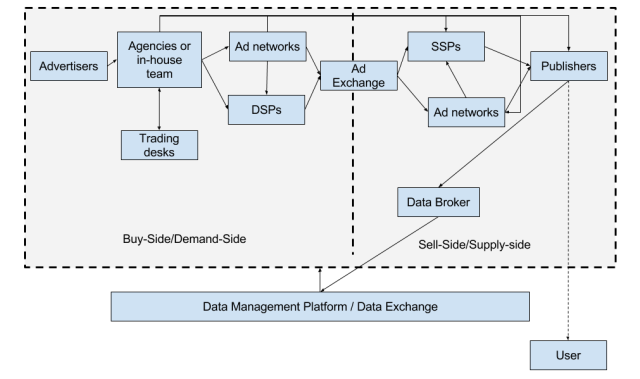
Advertisers are the folks who want to advertise their products and services.

Advertisers intend to “convert” people from a state of disinterestedness to a loyal customers who continually use the advertiser’s product or service. This is commonly abstracted as a marketing funnel given below.

Blog on advertising - figures

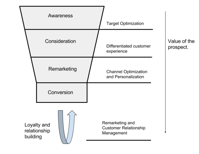
The top of the funnel comprises of prospects that are large in number and are selected based on customer segmentation and audience creation. Traditionally, this segment was addressed between the 1950s and the 90s through mass media like Television and Radio, and through mass mailers. As a prospect moves down the funnel, the possibility of a “conversion” is enhanced by personalizing the experience for the customer either online or offline, so that his/her specific needs are addressed. Lastly, a “converted” prospect who becomes a customer is a potential candidate for cross-selling offerings. Also, building a good relationship with him/her develops loyalty and helps business grow and sustain. E.g. Chevrolet, IPL, Tata, NFL, Nike

Agencies are companies that manage the spend of marketing money by designing, executing, and monitoring the ad-delivery experience for the advertiser. The agencies have to work in tight co-ordination with various stakeholders in the organization; sometimes, an in-house team performs the work of the agency as well.

With the sudden advent and necessity of using many technology “pieces” in delivering advertisements today, it has become a challenge for traditional ad-folks to keep pace and be relevant. As a result, holding companies of agencies have come up with the concept of trading desks that have the necessary skill sets siloed up in a separate organization that demands usage fee for its services. E.g. Havas Media, Omicom Group, WPP Group

Ad Networks are companies that specialize in matching advertisers to publishers. They operate on the model of arbitrage – by making the money that amounts to the difference of the publisher’s earnings and what the advertiser is willing to pay. These companies predate ad exchanges that are explained below. Ad networks traditionally suffered a lack of transparency, and sometimes, had unsold inventory that were sold to other ad-networks, leading to many “hops” for an advertiser to sometimes find inventory (known as daisy-chaining), leading to very high arbitrage. Such limitations of Ad Networks gave way to today’s Ad Exchanges, DSPs, DMPs, and SSPs. E.g. Tribal Fusion, Specific Media, Media.net, Conversant.

Ad Exchanges are companies that provide the necessary infrastructure for the publishers to sell their inventory through a bidding process to the advertisers. Since the market is fragmented with many ad-networks, publishers, and advertisers, publishers and advertisers often don’t directly connect to the ad-exchange and instead go through other companies called DSPs and SSPs, respectively. Today, most Ad Exchanges use a standard called OpenRTB [35] for their services. E.g. Google Ad Exchange, Yahoo! Ad Platform, Microsoft Advertising Exchange, MoPub, Nexage, Smaato

Demand-side Platforms (DSPs) serve the agencies (and hence the advertisers) by bidding for inventory. Their objective is to provide maximum return on the ad spend (ROAS) for the advertisers. They may do so by connecting to multiple Ad exchanges, networks, and SSPs. E.g. DataXu, MediaMath, Turn, Adnear

Supply-side Platforms (SSPs) serve the interests of the publishers by connecting them to various ad-exchanges and networks to sell their inventory for the best price.  E.g. Pubmatic and Rubicom

Data Management Platforms (DMPs) enable publishers and advertisers to store their data in a centralized system and re-use it for optimizing their actions (e.g bidding) or assets (e.g inventory placement). DMPs, as platforms are diverse and sometimes also enable storage of data (owned, derived, and bought) in a form that can be used for analyses, segmentation, and optimization. Also, they may act as a market place or a syndicate for various stakeholders to purchase, combine, and triangulate data. Generally, DMPs are of three kinds:

  1. Execution DMPs: that are geared towards certain types of channel and media with core DMP functions for use by DSPs.
  2. Pure-play DMPs: are the most common type in the market that in addition to performing core DMP functions of managing data, provide a rich interface to connect to various channels and media, syndicate various data sources, and also possibly a “data exchange” capability to purchase, sell, and integrate third-party data.
  3. Experience DMPs: that go beyond basic DMP functionality and provide tight integration with work-flows for personalization and “experience” management. By experience, we refer to the experience that a prospect would go through, as he/she moves through the conversion funnel.

Publishers are social media sites, websites, apps, televisions, radios, and other platforms that display advertisements to a prospect.  The prospect is called the user of the publisher’s services in the block diagram given above.

Lastly, it is to be noted that the publisher is also sometimes known as the seller and the advertiser is known as the buyer (of ad slots). Therefore the companies that represent the interests of the advertiser are on the supply-side or sellers’ side of the platform and those representing the interests of the advertisers are known to be on the demand-side or the buyers’ side of the platform.

A detailed list of companies falling of the advertising landscape is given in LUMAScape [3].

Technology abstractions

A modified version of various technology abstractions that have to be implemented, customized, or re-used for implementing a computational advertising solution from Dempster and Lee [2], is given below.

Blog on advertising - figures(2)

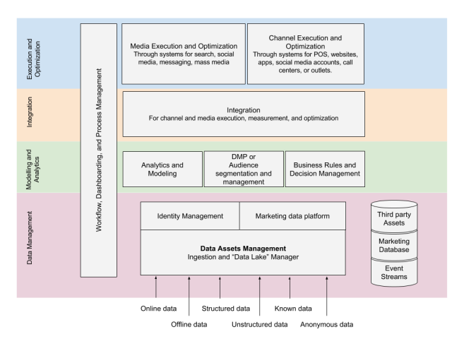
Data Assets Management refers to the ingestion and house keeping of various kinds of data available to the advertiser from third-party sources and owned assets. The data could be structured (questionnaires, relational tables from signup forms etc.) or unstructured (forum posts, contextual information from user pages, etc.), attributable to an individual user (aka known data) or anonymized.  Since the data collected at this step is heterogeneous, it could be abstracted as a “data lake” that is a central, comprehensive repository of all information. This information can be re-organized and normalized into traditional relation tables or other storage forms that assists with other functions such as analytics, decision making, and optimization. This can be called the Marketing data platform The data assets management layer is also used to manage Identities: i.e. associations of interactions at touch-points and behavioral data with unique identifiers, so that individual users or “look-alikes” can be identified and handled appropriately. Lastly, an important kind of data that has to be stored are event streams which are raw captures of interactions at touch-points for every user.  This is closely related to identity management and can be used to solve interesting problems like “attribution” which is discussed later in the article.

The data that has been ingested by the aforementioned Data Management layer is used for three purposes: for analysis and understanding, modeling and segmentation, and optimization.

Analysis could help understand the quantity and quality of data stored, performance of ad campaigns, and ad operations. Modeling refers extracting derived features, fixing missing data, and creating audience segments or groups that can be used for targeting. Lastly, optimization involves building business rules for creating a user experience, developing creatives, and coming up with strategies for spending money. While fine-grained experimentation, measurement, and optimization will have to happen while working with various media sources and channels, an overall strategy and decision making matrix is nevertheless necessary. All these three functions are shown in the Analytics and Modeling layer of the diagram.

Next, all the block diagrams discussed so far are usually developed by separate teams or are be based off of existing products. Their integration with other components for media and channel optimization such as DSPs, AdExchanges, web analytics providers, event stream trackers, etc. is therefore a distinct and important task and is referred to as Integration.

Lastly, we have two blocks that deal with media and channels, respectively.

The media execution and optimization block deals with various systems such as API driven Ad Networks, Ad Exchanges, Publisher APIs, and DMPs and algorithms for various tasks like price estimation, burn-rate estimation, and bidding decision making for RTB, and the like.

The channel execution and optimization block deals with various channels through which the advertiser wishes to engage with the prospect. They could be landing pages on a website, an app, a brick-and-mortar store, or a call center. The “experience” of a prospect as he goes down the conversion funnel has to be personalized and optimized to drive a conversion. This uses the outcome of the “creative” work of developing content and various techniques to “personalize” the experience of the user by exposing them to the right content and guiding them down the funnel.

Each abstraction discussed above is also closely tied to business processes, work flows, and manual interventions. All of this has to be managed through dashboards, work flow management systems, and the like.

Finally, The most important and yet often hardest to design is a conduit or the “glue” that ties all these blocks together to create an efficient and effective system for advertising.

Now, each of the abstractions described above expose several data science problems that are explored in the next section.

Organizational abstractions

For the sake of completeness, in a rather terse way, the general steps involved in an organization to setup the strategy for marketing is reproduced from [2], below.

Blog on advertising - figures(3)

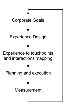
For a detailed treatment of how this can be achieved whilst avoiding common pitfalls like the creation of silos within teams, creating transformative changes in the organization, re-structuring to deal with the “new” interconnected nature of advertising without affecting team morale, etc. Please refer [2].

Data Science and Analytics Problems in Computational Advertising

In this section, relevant topics in computational advertising that involve the use of scientific and engineering tools are described. The discussion is further categorized based on the methodology required – quantitative and/or qualitative, and based on technological abstractions and stakeholders described in the previous section.

It has to be noted that although for the sake of clarity, the problems have been bucketed under certain headings, they are often interconnected and have an impact on other stakeholders or technology blocks.

  1. Customer Segmentation and Audience Creation

    Creating customer segments involves defining rules that can be applied to available data sources to extract “clusters”. This can be done in three ways:

    1. Qualitative data collection and analysis techniques such as structured and unstructured interviews, focus groups, and surveys [7, 8, 9].
    2. Based on processes that capture various important business metrics like lifetime-value (LTV) of a customer, cost of acquisition, data availability, and addressability of the segment [5] or business specific data [4].
    3. Using clustering methods in machine learning like K-means, Latent Dirchlet allocation, PLSA, and the like. [6]. In such cases, various cluster purity measures can be used to measure the robustness of segments [10].

    In all cases, segmentation is usually followed by identifying representative samples of each segment that can be described using features or words that are easy to understand: it could be the most representative rule, if decision trees are used, value of numeric variable used to generate the cluster, etc. These are known as personas. The segments may also be summarized with descriptive statistics (such as stating that 75% of the segment users used an iPhone everyday), into what are called profiles. These profiles and personas aid the creative process: to generate content and design experience for a customer at various touch points. It is also important to point out that segmentation often helps target ads to prospects at the top of the marketing funnel. A common pitfall is to over-rely on segments for targeting [2]. They should always be combined with contextual information. Additionally, the concept of assigning a data point to a segment need not be mutually exclusive; soft-assignments through propensity models may also be explored.

  2. Channel experience design

    Channel experience design is a creative activity and involves the design of a process document for capturing a creative brief. This may involve discussing with the stakeholders within an agency or the advertiser to identify:

    1. What the customer should feel, need, or do.
    2. The competitive advantage or the “selling edge” of the advertiser.
    3. Insights on the customer segment and their perspectives.
    4. Best ways to solicit customer response.

    All of these steps require a good understanding of the stakeholders involved, the right communication skills and knowledge of the best practices of various Qualitative research techniques, so that the process can be standardized as much as possible in the interest of efficiency (e.g. to allow for legal approvals of minor variants) and effectiveness (e.g. quality of segments wrt. conversion).

    Additionally, one has to abstract insights gained about the customer into a “decision diagram” that captures the rationale behind why a user would “convert”. As an example from [2], this could be through the identification of  the following chain of reactions: Brand Attributes (e.g. Offers, Convenient location) –> Brand Benefits (e.g. Good customer experience, Value for money) –> Personal Emotions (e.g. Feel valued, Confident) –> Personal Values (e.g. Pride, Peace of Mind).
    The resulting brief  should visualize and capture all the aforementioned content in a short 1-2 page document; it should be tested, through campaigns, focus groups, or the like. Preparing such a brief is an iterative process. In order to test various strategies that are outcomes of the brief, techniques like A/B [11], Multi-arm bandit [12], and the Taguchi method [13] can be used and are introduced again, as a part of the Content Optimization problem later.

  3. Budget Allocation

    The budget allocation problem deals with the amount and type of budget that should be allocated. It could happen along the following dimensions:

    1. Digital vs. Traditional advertising
    2. Publishers and ad-networks (e.g. Facebook vs. Google vs. Twitter) in computational advertising,
    3. Type of delivery, i.e. as a part of search results (search advertising), social media feeds (social media advertising), or as display banners (display advertising).
    4. Nature of contracts with the publisher, viz. Real-time Bidding, Programmatic Guaranteed or API-driven buying, or Guaranteed Media Buying (through what are known as Over-the-counter or OTC contracts). This is relevant as residual ad slots are often sold over RTB by a lot of publishers while allocating the most valuable slots through guaranteed contracts [2].
    5. Various parts of the conversion funnel: Prospecting vs. Remarketing vs. Cross-selling; Segment based targeting vs. Personalization lower down the funnel. This decision is complex and has to be based on addressability of market segments through these various types of advertising media, costs, and conversion rates in addition to organizational factors such as risk appetite, comfort with technology, and the like.
  4. Contract negotiation and Stakeholder’s Optimization

    Contracts are usually negotiated in two ways:

    1. Forward  contracts that are usually used with OTC contracts in which the advertiser purchases impressions in advance for some future time period. This is also called Guaranteed media buying. Alternatively they are also used transparent markets to purchase guaranteed ad slots, but through decisioning mechanisms that are controlled by the publisher (such as Yahoo! Guaranteed inventory or Facebook Inventory through an API developer)
    2. On the spot contracts that are used in markets that have transparent pricing through auctioning methods where the advertisements are bought immediately.

    In the case of forward contracts, using various mathematical optimization techniques are relevant from the perspectives of all stakeholders, namely, the ad exchanges, publishers, and advertisers. Each of them are discussed below:

    1. Ad Networks

      In the case of Ad networks, the objective of “optimization” would be to improve their revenues during auctioning. In this context, it is worthwhile to consider various auctioning models in vogue and that have phased out:

      1. 1st price negotiation and 1st price reservation are simple auctioning mechanisms that are used for manual selection of the most preferred contract or for implementing first-come-first-serve basis; they are relevant for OTC contracts).
      2. 2nd Price auctions are the most common auctions used in the context of the Real time bidding (RTB) industry. At a high level, they work in two steps; first, they combine  quality and relevance of the creative or the advertiser with the bid price to come up with a score; next, they use the price of the 2nd highest bid to determine the price the winner of the bid pays. A natural advantage of this method is that the quality and relevance can be factored into the bidding process (including possibly positional bias) and it also supports true RTB and pre-set bids (PSB). The generalized 2nd price auction [14] is the most adopted model nowadays in Ad Exchanges. It is briefly defined below due to its importance. Let’s say there are N ordered slots \{ 1, 2 \cdots N \} and K bidders. Let the probability of a slot in  position i being clicked be given by a_i with a_1 \ge a_1 \cdots \ge a_N. Let the bids of the K bidders and their “quality” scores be given by \{ b_1 \cdots b_K \} and \{ q_1 \cdots q_k \}. Then, the payment to the search engine for position i is given by p_i = \frac{b_{i+1} q_{i+1}}{q_i}A detailed discussion on its evolution in [14].
    2. Publishers and SSPs

      In the case of publishers or SSPs, the objective is to improve revenue whilst controlling relevance of advertisements. The discussion of problems can further be dissected based on the type of advertising: i.e. whether it is search, display, or social media advertising.

      In search advertising, relevance optimization amounts to determining (a) how many ads to show with a search result, (b) which ads to show (after bidding), and (c) where to show the ads. For (a), in literature, there are several studies involving eye tracking on pages [15, 16, 17, 18]. For (b) and (c), the problem is many-fold. Firstly, should an ad be displayed at all for a given search query or page? This is called the swing problem [19]. Secondly, how can the relevance score be computed? This has been done using a variety of techniques; with vector-space representation [20, 21] being used for extracting features and a variety of algorithms such as decision trees [25], SVMs [24], logistic regression [22], Bayesian Networks [23], and the like, for carrying out inference. These are tabulated well in [2]. Thirdly, relevance and revenue are sometimes at loggerheads. There is a need to achieve a certain number of impressions to generate revenue, but a lack of relevance can affect user experience and over a period of time, drive revenue down. So the aforementioned relevance improvement methods may have to be coupled with ways of also having sufficient addressability: This could be in the form of identifying relevant ads for uncommon queries (belonging to the long tail) using methods like query expansion using WordNet or by building models that optimize for total revenue whilst respecting daily budgets of bidders. This forms the basis for the AdWords problem described in [26]. In general, publishers in search advertising also have the advantage of exploiting the “semantic information” readily available in textual data.

      In the case of display advertising on mobile phones, videos, and display, an important problem is to again determine the best location for advertisements. In the case of videos, this problem is particularly complex; in literature, it has been addressed in a variety of ways such as identifying points of discontinuity, determining locations that are least obstructive, etc. The aforementioned swing problem, optimizing revenue and relevance are valid for these types of advertising as well.

      Social media advertising on the other hand provides a much more unique opportunity; while the swing, revenue and relevance problems are still relevant, the tend to transfer the targeting control to the advertiser or the buy-side. Forward contracts are still used, but the relevance parameters are usually preset, with the bid-optimization being managed by the publisher. The traditional relevance problem has to be re-defined in terms of how, where, and how frequently sponsored content may be interspersed with “feeds” to provide optimal revenue whilst not annoying a user: this may be done indirectly through CTR experiments and the like, or using various experiment design methodologies like multi-arm bandit.

      Lastly, the problem of revenue optimization is also closely tied to the issue of honoring contract requirements such as providing a certain number of impressions within a given time period or a certain number of actions, in the case of display advertising. This topic has also been investigated in the literature [30].

    3. Advertisers and DSPs

      Advertisers want their impressions delivered to the right audience at the lowest cost. DSPs may still want to improve their revenues (which might be a percentage of the ad spend), but they predominantly represent the advertiser’s interests. The following problems are relevant to them:

      Optimizing targeting: This involves choosing the right criteria to deploy advertisements. They can be of the following kinds:

      1. Behavioral: phone usage, web browsing history
      2. Attitudinal: emotions, preferences, needs
      3. Motivational: why behind the buy, underlying motivations
      4. Demographic: pertaining to age, location, affluence

      A special case for search advertising would be to map behavioral and attitudinal information to keywords and therefore, optimize keyword selection. As an example, in literature, linear programming, keyword bid statistics, and multi-arm bandit algorithms have been used [27, 28].  A related problem is determining target size [29]. The target size is important for an advertiser as it helps set an expectation on the budget that can be burnt in a given time for a given target criteria.

      The target optimization problem is further complicated in practice, by the need to burn money in a meaningful manner during the entire duration of a campaign. Various methods have been proposed to place good quality bids in literature [31, 33, 36, 37].
      Conceptually, the various dimensions that will have to be optimized jointly are:

      1. Criteria: keywords and/or behavioral, attitudinal, motivational, and demographic variables for improving the CTR, CPM, or any other metric that’s relevant.
      2. Burn-rate: requiring uniformity and minimization of the risk of pre-mature campaign termination.
      3. Burn-rate fluctuation: burn-rate to be relatively smooth and at the same time capture the traffic patterns; uniform burn rate is considered disadvantages because it disregards information about the time of the day when high quality and quantity impressions are possible.
      4. Re-targeting frequency: the number of times a single identity is shown an ad
      5. Creative choice: the possible choices could include different creative sizes(e.g. interstitial vs. banner), content, and types (e.g. video vs. banner vs. interactive) .

      The objective is to eventually develop a bidding function that positively impacts the KPI of the organization. This has also been discussed in literature [32].

      All in all, target optimization enables us to chose the right auctions to bid on; there are two sub problems in bidding: making a decision as to whether to bid or not, and if the decision is to bid, setting the bid price. These have to be solved as a part of the previous problem.


      Although unrelated to mathematical optimization, it is important to mention here that adding new sources of information, triangulating variables (such as geo IP mappings), and exploring new dimensions are equally important to improving targeting quality. This could be through the use of data management platforms that act as a syndication of data sources. Also, it is important to understand three kinds of data commonly referred to in advertising:

      1. First-party data: is the data owned by the stakeholder that we’re talking about. e.g. CRM database of an advertiser is his first-party data.
      2. Second-party data: is the first-party data of someone else. For example, buying Facebook’s data would amount to purchasing second-party data.
      3. Third-party data: is someone else’s data sold by an intermediary.

      For a description of how a DMP works, the reader is pointed to [34].

  5. Content Optimization

    Content optimization happens at two places: Firstly, the creative content has to be optimized through an iterative process. This has to be documented in the brief.  Secondly and most importantly, the content in the channels of the advertiser has to be worked upon to “create” the experience that has been designed for the prospect. This amounts to building “personalization”. Personalization is defined as “the enablement of dynamic insertion, customization, or suggestion of content in any format that is relevant to the individual user, based on the individual user’s implicit behavior and preferences, and explicit customer provided information”[2].

    At every touchpoint on the channel, the user defines a clear a topic: such as product, services, loyalty, up-sell, cross-sell, or general questions. It is therefore the objective of “personalization” to address such needs of the user in context, with specificity.  Concretely, for instance, the choice of offer may be different for a returning customer and a prospect who is at the “consideration” part of the marketing funnel. The choice of offers to be shown, its positioning on the website, and surrounding content will have to be optimized using various techniques in experiment design such as A/B testing, multi-arm bandit, the Taguchi method, and the like. This is a an iterative process and involves analyzing web analytics logs and event streams to identify drop-offs for various strategies (chosen through experiments), time spent on pages, etc.  in order to further improve conversion rates.

  6. Measurement and Analysis

    The first and the foremost problem of an advertising solution is being able to measure the performance of the various technological abstractions that was described in the previous section. For example, what is the accuracy of identity matching? what are the false positive and false negative rates? What is the accuracy of the data provided by the DMP? How well is a targeting criteria performing? What is the LTV of a customer? What is the value of an impression? How good is the outcome of an advertising campaign? Why are prospects dropping off of a conversion funnel? Why is there a churn?

    While the list of questions given above are not exhaustive, they are indicative of the absolute necessity of defining metrics at various stages and measuring them. Such measurements may also be necessary in a lot of the optimization and other data science problems discussed above. Some of the abstractions may not be “measurable” (e.g. customer segments), in which case, they may have to be studied in depth as to whether such abstractions make sense or if their quality has to be measured indirectly. All in all, a comprehensive plan for a measurement rig is absolutely essential.

    In addition to making measurements, it is also essential to make measurements comparable where it make sense. The pricing for an impression, for example, is given through metrics like Cost-per-mille (CPM), Cost-per-Click (CPC), Cost-per-acquisition (CPA), and so on. In the case of bids, the ad exhange uses what is known as a dynamic CPM with the CPM varying between bids. In order to get the bid value to the same currency, a DSP or an advertiser may chose to normalize it eCPM (or effective CPM that normalizes CPM by the expected number of impressions).

    Apart from these fundamental challenges with making the entire solution measurable at various stages, the following measurement-related problems require data-driven solutions.

    1. Fraud detection

      Internet advertising fraud is a major loss of revenue for advertisers. Recent reports suggest that ad frauds in 2016 amount to about 7.6 Billion USD! [38] Also, some sources suggest that up to 60% of ad traffic constitutes fraud [39]. Fraud happens because of fake clicks on advertisements that are a irrecoverable cost to the advertiser.

      Various methods to detect or prevent fraud has been presented in literature by different stake holders such as advertisers and ad networks [40, 41, 42]; nevertheless, it has been broadly acknowledged, both in media and research that this is a pervasive and tough problem to solve.

    2. Attribution

      Attribution refers to the identification of the cause for a conversion or an interaction on a channel. Attribution is important as it enables us to understand and optimize user experience and therefore lead to more conversions. It also helps us allocate the right advertising budget to various portions of the conversion funnel. The simplest strategy for attribution is known as “last-touch” attribution that assigns the complete cause for a conversion to be the most recent interaction. This leads to erroneous results when the marketing solution involves, say, remarketing messages and various personalization steps, that eventually lead to a conversion. As an alternative, more complicated attribution models have been proposed in literature that assign attribution to multiple sources using techniques from game theory,  time-series models, aggregations, and machine learning and are generally called “fractional attribution” or “multi-touch attribution” models [43, 44, 45, 46].

    3. Cross-device identification

      With the large always-on-mobile population as well as the pervasiveness of the websites and social media, and the possible existence of rich offline data collected by advertisers, it is becomes imperative that one is able to triangulate all of these data sources to identify individual users. However, this is a challenge due to the following reasons:

      1. The creation of “Walled Gardens” by large publishers that limit exposure of user identities to the advertiser in the absence of an interaction.
      2. The use of multiple devices by a single user
      3. The use of identities that are unique to a device (e.g. IDFA or Android ID) and the lack of cookie management in smartphones and tablets
      4. The possibility of clearing a cookie by the user, and
      5. Popularity of browser addons like AdBlocker, Ghostery, etc.
      6. Lack of sufficient identity information or ambiguity in the case of offline to online data matching.

      As a result, identifying a user across devices or websites, where not directly possible, is sometimes attempted using probabilistic methods. Such methods rely on similarity of or correlation between variables to match users. The accuracy of such systems have not been extensively studied (or made available as public literature) although a robust system can potentially open up great possibilities.

  7. User Perceptions of Advertising

    One of the most important questions that an advertiser has to answer for himself is about the perception of advertisements by a user along several dimensions: whether it is relevant or annoying, whether it is visible or obscurely placed, and whether the targeting and data collection mechanisms used by the advertiser (and possibly the publisher) are perceived to be privacy-sensitive.

    Here, the importance of privacy needs to be underscored and qualitative studies in literature have also explored this [47]. The control of privacy may also have to be given to the user (as evidenced by recent changes to Facebook settings), the use of PII avoided, privacy policy written in simple language (as have many companies including Facebook and Google have) etc. This is an ongoing and active research area, given its subjective nature and continually changing user attitudes. Understanding them along with government regulations are very essential for both, ensuring a compliant and acceptable solution and to influence policy making as a stakeholder.

    Lastly, with the advent and popularity of various plugins and add-ons on phones and browsers that disable advertisements (like Ghostery, AdBlock Plus, etc.), it is also imperative to understand user attitudes to advertising in various contexts through qualitative and quantitative research methods.

This brings us to the end of the rather longish article. Do share feedback and comments!

References

  • [1] Shaui Yuan, Ahmad Zainal Abidin, Marc Sloan, Jun Wang. Internet Advertising: An interplay among Advertisers, Online Publishers, Ad Exchanges, and Web Users. Preprint. Information Processing and Managment. 2012.
  • [2] Craig Dempster, John Lee. The raise of the Platform Marketer: Preformance Marketing with Google, Facebook, and Twitter plus High-Growth Digital Advertising Platforms. Wiley and Sons. 2015.
  • [3] Luma Partners. LumaSCAPE. http://www.lumapartners.com/lumascapes/display-ad-tech-lumascape/. Accessed 21 Jun 2016.
  • [4] Thorsten Teichert, Edlira Shehu, Iwan von Wartburg. Customer segmentation revisited: The case of the airline industry. Transporation Research. pp. 227-242. 2008.
  • [5] Su-Yeon Kim, Tae-Soo Jung, Eui-Ho Suh, Hyun-Seok Hwang. Customer segmentation and strategy development based on customer lifetime value: A case study. Vol. 31. pp. 101-107. 2006.
  • [6] Wu X, Yan J, Liu N, Yan S, Chen Y, Chen Z. Probabilistic latent semantic
    user segmentation for behavioral targeted advertising. In: Proceedings of the
    3rd International Workshop on Data Mining and Audience Intelligence for
    Advertising. 2009. p. 10–7.
  • [7] Jenny Kitzinger. Introducing Focus Groups. BMJ. Vol. 311. pp. 299-302. 1995.
  • [8] Annabel Bhamani Kajornboon. Using interviews as research instruments. Technical Report. Chulalongkorn University. http://www.culi.chula.ac.th/Research/e-Journal/bod/Annabel.pdf. Accessed June 20, 2016.
  • [9] Rosalind Edwards, Janet Holland. What is qualitative interviewing? “What is” Research Method Series. Bloomsbury. 2013.
  • [10] Sabine Schulte im Walde. Chapter 4: Clustering Algorithms and Evaluation. Experiments on the Automatic Induction of German Semantic Verb Classes. Institut für Maschinelle Sprachverarbeitung, Universität Stuttgart, June 2003.
  • [11] Wikipedia. A/B Testing. https://en.wikipedia.org/wiki/A/B_testing . Retrieved June 20, 2016.
  • [12] Joann es Vermorel, Mehryar Mohri. Multi-armed Bandit Algorithms and Empirical Evaluation. ECML. pp. 437-448. 2005.
  • [13] Roy R. A primer on taguchi method. Society of Manufacturing Engineers, 1990.
  • [14] G Aggarwal, S Muthukrishnan. Theory of sponsored search auctions. In: Foun-
    dations of Computer Science, 2008. FOCS’08. IEEE 49th Annual IEEE Sym-
    posium on. IEEE; 2008. p. 7–.
  • [15] Granka L, Joachims T, Gay G. Eye-tracking analysis of user behavior in www
    search. In: Proceedings of the 27th ACM SIGIR Conference on Information
    Retrieval. ACM; 2004. p. 478–9.
  • [16] Granka L, Joachims T, Gay G. Eye-tracking analysis of user behavior in www
    search. In: Proceedings of the 27th ACM SIGIR Conference on Information
    Retrieval. ACM; 2004. p. 478–9.
  • [17] Enquiro . Barriers on a search results page. 2008.
  • [18] Gord Hotchkiss SA, Edwards G. Google eye tracking report. http://pages.
    enquiro.com/whitepaper-enquiro-eye-tracking-report-I-google.
    html (last visited 13/12/2011); 2005.
  • [19] Broder A, Ciaramita M, Fontoura M, Gabrilovich E, Josifovski V, Metzler D,
    Murdock V, Plachouras V. To swing or not to swing: learning when (not) to
    advertise. In: Proceeding of the 17th ACM Conference on Information and
    knowledge Management, CIKM. ACM; 2008a. p. 1003–12.
  • [20] Broder A, Ciccolo P, Fontoura M, Gabrilovich E, Josifovski V, Riedel L.
    Search advertising using web relevance feedback. In: Proceedings of the 17th
    ACM Conference on Information and Knowledge Management, CIKM. ACM;
    2008b. p. 1013–22.
  • [21] Broder A, Ciccolo P, Gabrilovich E, Josifovski V, Metzler D, Riedel L, Yuan J.
    Online expansion of rare queries for sponsored search. In: Proceedings of the
    18th International Conference on World Wide Web. 2009. p. 511–20.
  • [22] Hillard D, Schroedl S, Manavoglu E, Raghavan H, Leggetter C. Improving
    ad relevance in sponsored search. In: Proceedings of the 3rd International
    Conference on Web Search and Data Mining. 2010. p. 361–70.
  • [23] Radlinski F, Broder A, Ciccolo P, Gabrilovich E, Josifovski V, Riedel L. Op-
    timizing relevance and revenue in ad search: a query substitution approach.
    In: Proceedings of the 31st ACM SIGIR on Information Retrieval. 2008. p.
    403–10.
  • [24] Richardson M, Dominowska E, Ragno R. Predicting clicks: estimating the
    click-through rate for new ads. In: Proceedings of the 16th International
    Conference on World Wide Web. 2007. p. 521–30.
  • [25] Neto BR, Cristo M, Golgher PB, de Moura ES. Impedance coupling in content-
    targeted advertising. In: Proceedings of the 28th ACM SIGIR on Information
    Retrieval. 2005. p. 496–503.
  • [26] Mehta A, Saberi A, Vazirani UV, Vazirani VV. Adwords and generalized on-
    line matching. In: Proceedings of the 46th Annual IEEE Symposium on
    Foundations of Computer Science. 2005. p. 264–73.
  • [27] Even-Dar E, Mirrokni VS, Muthukrishnan S, Mansour Y, Nadav U. Bid opti-
    mization for broad match ad auctions. In: Proceedings of the 18th Interna-
    tional Conference on World Wide Web. 2009. p. 231–40.
  • [28] Rusmevichientong P, Williamson DP. An adaptive algorithm for selecting prof-
    itable keywords for search-based advertising services. In: Proceedings of the
    7th ACM Conference on Electronic Commerce. 2006. p. 260–9.
    [29] S. Muthukrishnan. Internet Ad Auctions: Insights and Directions. ICALP. 2008. pp. 14-23
  • [30] Korula, Nitish, Vahab Mirrokni, and Hamid Nazerzadeh. “Optimizing display advertising markets: Challenges and directions.” Available at SSRN 2623163 (2015).
  • [31] Kuang-Chih Lee,Ali Jalali, Ali Dasdan, Real Time Bid Optimization with Smooth Budget Delivery in Online Advertising. ADKDD 2013.
  • [32] Weinan Zhang, Shuai Yuan, Jun Wang. Optimal Real-Time Bidding for Display Advertising. KDD 2014.
  • [33] Shuai Yuan, Jun Wang, Xiaoxue Zhao. Real-time Bidding for Online Advertising: Measurement and Analysis. ADKDD 2013.
  • [34] Hazem Elmeleegy, Yinan Li, Yan Qi, Peter Wilmot, Mingxi Wu, Santanu Kolay, Ali Dasdan. Overview of Turn Data Management Platform for Digital Advertising. Proceedings of the VLDB Endowment, Vol. 6, No. 11. 2013.
  • [35] IAB. OpenRTB Specification. http://www.iab.com/wp-content/uploads/2015/05/OpenRTB_API_Specification_Version_2_3_1.pdf . Accessed June 22, 2016.
  • [36] Shahriar Shariat, Burkay Orten, Ali Dasdan. Online Model Evaluation in a Large-Scale Computational Advertising Platform. arXiv:1508.07678v1 CS:AI. 2015.
  • [37] Kuang-chih Lee, Burkay Orten, Ali Dasdan, Wentong Li. Estimating Conversion Rate in Display Advertising from Past Performance Data. KDD 2012.
  • [38] George Slefo. Ad Fraud Will Cost $7.2 Billion in 2016, ANA Says, Up Nearly $1 Billion.  http://www.adageindia.in/digital/ad-fraud-will-cost-7-2-billion-in-2016-ana-says-up-nearly-1-billion/articleshow/50647542.cms . Accessed June 22, 2016.
  • [39] Mathew Ingram. There’s a ticking time bomb inside the online advertising market.
    http://fortune.com/2015/07/01/online-advertising-fraud/ . Accessed June 22, 2016.
  • [40] Linfeng Zhang and Yong Guan. Detecting Click Fraud in Pay-Per-Click Streams of Online Advertising Networks. The 28th International Conference on Distributed Computing Systems. 2008.
  • [41] Hamed Haddadi. Fighting Online Click-Fraud Using Bluff Ads. arXiv:1002.2353v1 CS: CR. 2010.
  • [42] Neil Daswani, Chris Mysen, Vinay Rao, Stephen Weis,. Online Advertising Fraud. Book Chapter from Crimeware. Symantic Press. 2008.
  • [43] Ron Berman. Beyond the Last Touch: Attribution in Online Advertising. Technical Report. 2015.
  • [44] Pavel Kireyev, Koen Pauwels, Sunil Gupta. Do display ads influence search? Attribution and dynamics in online advertising. International Journal of Research in Marketing. 2015.
  • [45] Sahin Cem Geyik, Abhishek Saxena, Ali Dasdan. Multi-Touch Attribution Based Budget Allocation in Online Advertising. ADKDD 2014.
  • [46] Xuhui Shao,Lexin Li. Data-driven Multi-touch Attribution Models. KDD 2011.
  • [47]Predrag Klasnja, Sunny Consolvo, Tanzeem Choudhury, Richard Beckwith, and Jeffrey Hightower. 2009. Exploring Privacy Concerns about Personal Sensing. In Proceedings of the 7th International Conference on Pervasive Computing (Pervasive ’09), Hideyuki Tokuda, Michael Beigl, Adrian Friday, A. J. Brush, and Yoshito Tobe (Eds.). Springer-Verlag, Berlin, Heidelberg, 176-183.
Posted in Analytics, Data Science | Tagged , , | Leave a comment

A Survey of Big-Data Companies

This is a little dated, but posting it FWIW…. PDF

If somebody is interested to update and beautify it, will be happy to share the data. Please buzz me for this at gokul@quaintscience.com

Thanks!!

Posted in Data Science | Tagged , | Leave a comment